Week 9 - FVM Literature Review

Abstract: This study illustrate about Finite Volume Method (FVM). And differences between finite difference method (FDM) & finite volume method (FVM). It includes details for interpolation schemes and flux limiters in FVM by taking a 1D linear heat conduction equation as an example.

Finite Volume Method (FVM):

• The FVM is a method for representing and evaluating partial differential equations (PDEs) in the form of algebraic equations similar to FDM and FEM.
• The geometry is discretized into smaller control volumes in which the governing equations are conserved.
• FDM discretizes into individual nodes but FVM discretizes into control volume surrounding the nodes.
• In FVM the governing PDEs were integrated over discretized control volumes.
• The divergence theorem is applied here to convert volume integrals to surface into integrals.
• Surface integrals are used to evaluate the fluxes at finite volumes.

Difference between FVM and FDM:

FDM:

• FDM discretization is based upon the differential form of the PDE to be solved.
• Each derivative is replaced with an approximate difference formula.
• The computational domain is usually divided into grid points, and the solution will be obtained at each nodal point.
• The FDM is easiest to understand when the physical grid is Cartesian.
• FVM discretization is based upon an integral form of the PDE to be solved
• The PDE is written in a form that can be solved for a given finite volume.
• The computational domain is discretized into finite volumes and then for every volume, the governing equations are solved. The resulting system of equations usually involves fluxes of the conserved variable, and thus the calculation of fluxes is very important in FVM.
• The basic advantage of this method over FDM is it does not require the use of structured grids, and the effort to convert the given mesh into a structured numerical grid internally is completely avoided.

Need for Interpolation schemes and flux limiters in the FVM technique.

1D - Linear heat conduction equation:

`d/dx(alpha.(dT)/dx) +S = 0`

where T -Temperature

S -Source term

`alpha` -Thermal diffusivity

The portion of the domain discretized is shown below

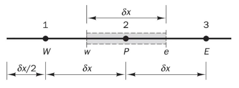
As we know 1D - linear conduction governing equation mentioned above is valid at every point in our domain. So it is valid for the entire control volume.

Here control volume with P as a centre is taken to be our point of interest. So we integrate the 1D linear conduction equation over this control volume with the limit w to e.

`int_e^wd/dx(alpha.(dT)/dx)dv +int_e^wSdv = 0`

`int_e^wd/dx(alpha.(dT)/dx)Adx +int_e^wSdv = 0`

`[alpha.A(dT)/dx]_w^e +int_w^eSdv = 0`

`[alpha.A(dT)/dx]_w^e +barSdv = 0`

`[alpha.A(dT)/dx]_e -[alpha.A(dT)/dx]_w+barSdv = 0`

`alpha.A[(T_e-T_p)/(deltax)] -alpha.A[(T_p-T_w)/(deltax)]+barSdv = 0`

Here the source term is function of temperature so it is desirable to consider this dependency in formulating discretized equation. We should account this dependency in a linear fashion since these discretized equations will be solved using linear algebraic equations.

`barS=S_c+SpTp`

where

`S_c`-Constant part

`S_p`-Coeffient of `T_p`

Interpolation scheme:

To evaluate the surface integrals and volume integrals in FVM, we need values at locations otherthan the centre nodes of the control volumes. These values can be found using interpolation scheme. These interpolation schemes are of different types

1. Central differencing scheme

2. Upwind differencing scheme

3. Quadratic upwind differencing scheme

4. Hybrid interpolation scheme

5. Total variation diminishing scheme

Flux limiters:

Flux limiters are used in high-resolution schemes – numerical schemes used to solve problems in science and engineering, particularly fluid dynamics, described by partial differential equations (PDE's).

They are used in high-resolution schemes, such as the MUSCL scheme, to avoid the spurious oscillations (wiggles) that would otherwise occur with high order spatial discretization schemes due to shocks, discontinuities or sharp changes in the solution domain.

The main idea behind the construction of flux limiter schemes is to limit the spatial derivatives to realistic values – for scientific and engineering problems this usually means physically realizable and meaningful values.

For smoothly changing waves, the flux limiters do not operate and the spatial derivatives can be represented by higher order approximations without introducing spurious oscillations.