Literature Review of Finite Volume Method (FVM)
Objective:
What is the Finite Volume Method(FVM), write down the major differences between FDM & FVM. Also, describe the need for interpolation schemes and flux limiters in FVM. You can use the 1D linear heat conduction equation as an example.
Solution:
The Finite Volume Method (FVM) is a discretization method for the approximation of a single or a system of PDE expressing the conservation, or balance, of one or more quantities. These partial differential equations (PDEs) are often called conservation laws; they may be of different nature, e.g. elliptic, parabolic or hyperbolic, and they are used as models in a wide number of fields, including physics, biophysics, chemistry, image processing, finance, dynamic reliability. They describe the relations between partial derivatives of unknown fields such as temperature, concentration, pressure, molar fraction, the density of electrons, or probability density function, with respect to variables within the domain (space, time,...) under consideration.
As in the finite element method, a mesh is constructed, which consists in a partition of the domain where the space variable lives. The elements of the mesh are called control volumes. The integration of the PDE over each control volume results in a balanced equation. The set of balance equations is then discretized with respect to a set of discrete unknowns. The main issue is the discretization of the fluxes at the boundaries of each control volume: in order for the FVM to be efficient, the numerical fluxes are generally
- conservative, i.e. the flux entering a control volume from its neighbor must be the opposite of the one entering the neighbor from the control volume,
- consistent, i.e. the numerical flux of a regular function interpolation tends to the continuous flux as the mesh size vanishes.
It is sometimes possible to discretize the fluxes at the boundaries of the control volume by the finite difference method (FDM). In this case, the method has often been referred to as a finite difference method or conservative finite difference method. The specificity of the FVM with respect to the FDM is that the discretization is performed on the local balance equations, rather than the PDE: the fluxes on boundaries of the control volumes are discretized, rather than the continuous differential operator.
The resulting system of discrete equations depends on a discrete (finite) set of unknowns, and may be either linear or nonlinear, depending on the original problem itself; this system is then solved exactly or approximately, using for example direct or iterative solvers in the case of linear equations and fixed point or Newton-type methods in the case of nonlinear equations.
Let us emphasize that there is no systematic way to derive the discrete system from the continuous one; in fact, the physical or engineering knowledge of the problem is in many cases the key ingredient in order to obtain a scheme that satisfies the expected properties of accuracy, robustness, and computational cost. Let us mention that in some cases, the engineering problem is initially set at a discrete level: the model consists of a set of discrete balance equations and therefore written as a finite volume scheme, and the continuous model of the problem is not explicitly given.
Many of these issues have often been addressed in computational fluid mechanics. A review of the schemes for the discretization of the compressible and incompressible Navier-Stokes and Euler equations may be found in e.g. Wesseling and Feistauer. The FVM has also been very early introduced in the framework of oil reservoir engineering.
Fundamental principle:
Consider the following PDE under conservative form
where the space variable x belongs to the domain Ω⊂Rd (d is the space dimension, greater or equal to 1), and the time variable t belongs to some time interval [0, T], with T>0. The scalar function A, defined in Ω×[0, T], expresses the density of some quantity, and ∂tA denotes its time derivative. The function F, defined in Ω×[0, T] and valued in Rd, express the flux of this quantity, and ∇⋅F denotes its space divergence. The function S, defined in Ω×[0, T] and valued in R, denotes some source term. Some initial condition A(x,0)=Aini(x) for x∈Ω is imposed, where the function Aini is defined in Ω and valued in R, as well as some boundary conditions, which depend on the considered equation. Note that the functions A and F are not necessarily regular, so that the derivatives involved in 1 may be weak derivatives.11111
These functions A, F , S are assumed to be related to a set of unknown fields (uj)j=1,…, N, where uj is an unknown function defined from Ω×[0, T] to R . Such relationships may for instance be written as
where the functions A , S and F are given. Classical examples with N=1 (we then denote by u the unique component u1), are:
- the heat equation which corresponds to A(x,t)=u(x,t) , and u is the temperature; F(x,t)=−Λ(x)∇u(x,t) (where for any x∈Rd , Λ(x) is a linear operator from Rd to Rd), S(x,t)=S(x,t) ;
- the Poisson equation, which is the steady version of the heat equations A(x,t)=0 , F(x,t)=−Λ(x)∇u(x) , S(x,t)=S(x) ;
- the linear convection equation A(x,t)=u(x,t) , F(x,t)=u(x,t)V(x,t) where V is a function defined from Ω¯¯¯×[0,T] to Rd , u is, say, a concentration, and V its transport velocity.
The domain Ω is partitioned into a mesh, denoted by M . In general, the mesh M is a finite family of nonoverlapping subsets of Ω, which satisfy a number of regularity properties; some of these properties are needed for the definition of the scheme, while others are required to establish the precision and the convergence of the method, depending on the type of term that needs to be discretized. The elements of M, denoted by K, L, are called the control volumes; the measure of a control volume K (its length if d=1, area if d=2, volume if d=3) is denoted by |K|. The boundary ∂K of each control volume K is partitioned into the finite set EK, called the set of the faces (d=3) or edges (d=2) or extremities (d=1) of K . An element σ of EK is either located on the boundary of Ω or belongs to EK∩EL where K and L are two adjacent control volumes.

The (d−1)-dimensional measure of a face σ∈EK (its length if d=2, area if d=3) is denoted by |σ|. A strictly increasing finite sequence t(0)=0<t(1)<…<t(N)=T is defined for the time discretization, and one denotes δt(n)=t(n)−t(n−1) , for n=1,…,N . The classical finite volume approximation of (1) relies on the approximation of the balance equations on the control volumes between time t(n−1) and t(n) (in fact, the balance equations usually precede the continuous equation 1 in the derivation of the model; this is the reason why, in several engineering applications, the FVM is applied directly to the discrete balance equations without any knowledge of the continuous equations). These balance equations may be obtained by integrating (1) on K×[t(n−1),t(n)] and using the divergence formula
where ds(x) denotes the integration with respect to the (d−1)-dimensional measure of the boundary and nK,σ(x) the unit vector normal to σ at point x, outward to K . The FV scheme is a discretization of the above balance equation and may be written as
where
F(n)K,σ is an approximation of ϕ(n)K,σ=1δt(n)|σ|∫t(n)t(n−1)∫σF(x,t)⋅nK,σ(x)ds(x)dt,
and
S(n)K is an approximation of 1δt(n)|K|∫t(n)t(n−1)∫KS(x,t)dxdt.
For a face σ common to two control volumes K and L , since nK,σ(x)+nL,σ(x)=0 for x∈σ , the normal fluxes in the original problem satisfy the conservation property ϕ(n)K,σ+ϕ(n)L,σ=0 . A discrete version of this property of conservation is then required
This relation is one of the pillars of the classical FVM; moreover, it is crucial in the mathematical analysis for proving convergence properties.
Discrete expressions in terms of discrete unknowns must then be provided for the terms A(n)K , F(n)K,σ and S(n)K . These discrete unknowns are usually expected to be approximations of the unknown functions (uj)j=1,…,N at different locations (grid blocks, faces, vertices,...) and times: hence u(n)j,K (resp. u(n)j,σ) denotes the approximation of function uj in control volume K (resp. at face σ) at time t(n) . For example, considering the case given in (2), it is generally possible to simply use the function A to define A(n)K , using an expression such as
A(n)K=1|K|∫KA(u(n)1,K,…,u(n)N,K,x,t(n))dx.
It is generally less simple to derive from (2) an expression for F(n)K,σ with respect to the discrete variables since there is no systematic method to use the function F which ensures accuracy and stability on general grids; the discretization of diffusion and convection fluxes are discussed below.
The arguments for the discrete expression of S(n)K are generally u(m)j,K ,..., m=n or n−1 .
differences between FDM & FVM
Finite-Difference Method: Advantages and Disadvantages
The finite-difference method is defined dimension per dimension; this makes it easy to increase the “element order” to get higher-order accuracy. If you can fit the simulation in a rectangular or box-shaped geometry using a regular grid, efficient implementations are much easier than for finite-element and finite-volume methods. Regular grids are useful for very-large-scale simulations on supercomputers often used in, as mentioned before, meteorological, seismological, and astrophysical simulations.
With the finite-difference method, you may easily run into problems handling curved boundaries for the purpose of defining the boundary conditions. Boundary conditions are needed to truncate the computational domain. They represent communication with the surrounding world, which is the part that you do not want to be included in your simulation. If one can overcome the boundary-condition problem on curved boundaries, the method gives very efficient and high-quality results.
For computations that need high accuracy, the extra effort in making boundary-fitted meshes and the associated complications of such meshes for the implementation may be worth it. Examples include Formula 1 car computational-fluid-dynamic (CFD) simulations and space-shuttle CFD simulations. The finite-difference method is more difficult to use for handling material discontinuities. In addition, it does not lend itself to local grid refinement or anything similar to “adaptive mesh refinement.” This may be needed to resolve local rapid variations in solutions such as around a corner of a complex shape, as described earlier.
Finite-Volume Method: Advantages and Disadvantages
The finite-volume method is a natural choice for CFD problems since the partial differential equations you have to solve for CFD are conservation laws. However, both finite differences and finite elements can also be used for CFD. Efficient technology for CFD with the finite-element method has become increasingly popular over the last 10 to 15 years. Techniques for CFD with the finite-difference and finite-volume method have been known and used much longer.
The finite-volume method’s strength is that it only needs to do flux evaluation for the cell boundaries. This also holds for nonlinear problems, which makes it extra powerful for robust handling of (nonlinear) conservation laws appearing in transport problems.
The local accuracy of the finite-volume method, such as close to a corner of interest, can be increased by refining the mesh around that corner, similar to the finite-element method. However, the functions that approximate the solution when using the finite-volume method cannot be easily made of higher-order. This is a disadvantage of the finite-volume method compared to the finite-element and finite-difference methods.
Need for interpolation schemes and flux limiters in FVM.
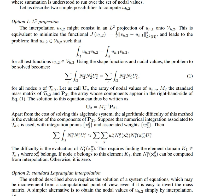
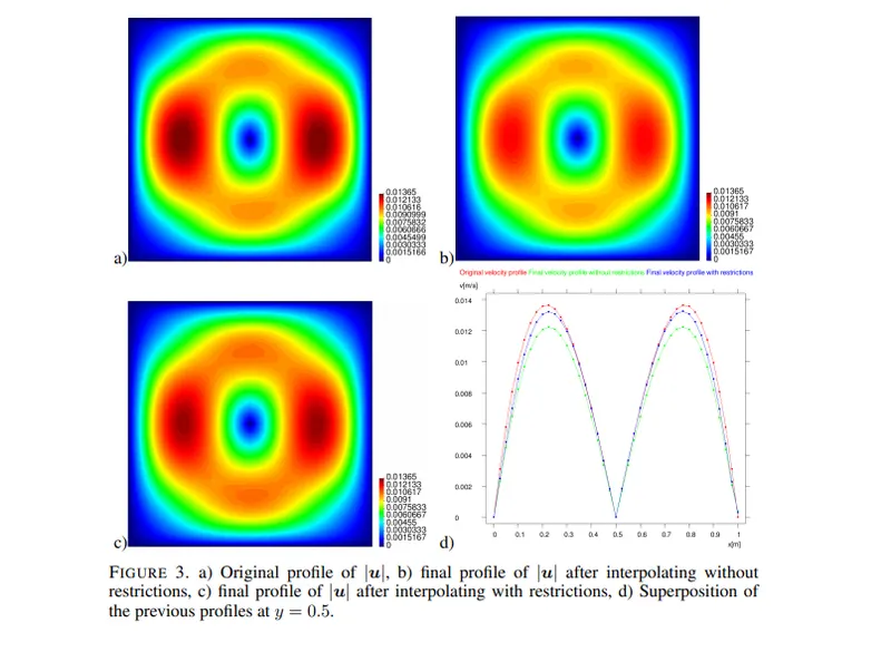
Let us consider a finite element partition Th,1 of a domain Ω ⊂ Rd, d >= 1, and a discrete solution uh,1 of an arbitrary problem defined in the subspace of functions Vh,1 ⊂ V, where V is the space of functions where the continuous solution lives. For the sake of conciseness,
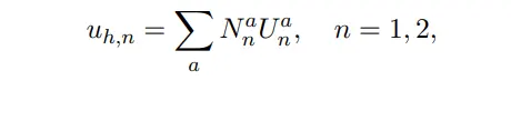
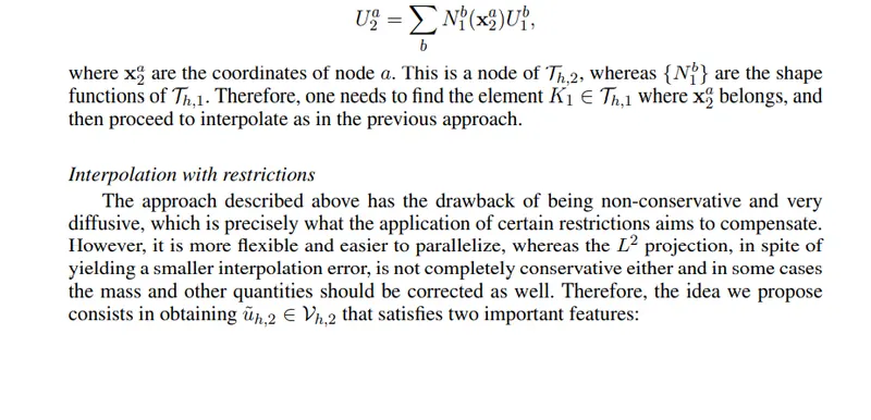
we will consider scalar functions in this section. Given another finite element partition Th,2 of the same domain, the objective is to construct uh,2 from uh,1 with the same approximation properties to the continuous solution as uh,1. We will call uh,2 the interpolation of uh,1 on Th,2 (see Fig. 1), and Vh,2 the corresponding finite element space. In order to simplify the notation for the rest of the paper, the finite element functions will be expressed in terms of the shape functions of each finite element partition, which will be denoted as {Na n}, where n = 1, 2 refers to the mesh and the superscript to the nodes, so that a will run from 1 to the number of nodes of each mesh. Denoting by Uan the corresponding nodal values and assuming a standard Lagrangian interpolation, we may write
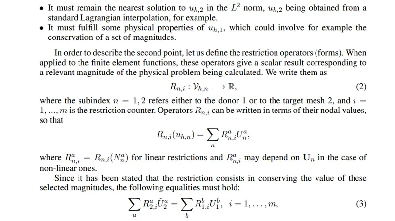
where U˜
2 denotes the nodal values associated with u˜h,2. The computational domain Ω remains the same for all stages of the process since the interpolation process is completely static although the simulation considers a dynamic domain. In some cases, only a part of the domain needs to be interpolated, for example in the case of fluid-structure interaction (FSI) problems, where the values at the interface must be exchanged between both subdomains. This scenario will not be considered in the present work. Although this method is only presented for some particular flow problems, it can be extended to other physical problems. For example, the formulation could be extended to flows with free surfaces in a straightforward way by restricting the constraints to the flow subdomain, which would require supplemental integration, Codina et al. (2009). Problems in
which the restrictions are inequalities rather than equalities could also be treated by embedding the scheme in an iterative loop that requires to solve a sequence of problems with equality constraints, as it is done in optimization; these inequality restrictions are found for example
in plasticity problems, where the stresses are required to be admissible, Brancherie et al. (2006). This last example requires a further extension consisting in posing the restriction in terms of variables defined at the numerical integration points, such as internal variables like
plastic multipliers or damage; it is only required to be able to express these variables in terms of the nodal unknowns of the problem and proceed as we propose here. At this point, it is important to distinguish the current method from the mortar method, Bernardi (1994). Unlike the present method, the mortar method consists of a domain decomposition technique that performs a L 2 projection along with an interface between nonmatching grids satisfying adequate matching conditions. The restriction of these fluxes might be performed with Lagrange multipliers. In our case, the interpolation is performed point by point and the restrictions affect the whole domain. 2.2. Application to linear restrictions Let us develop the concept introduced above in the case in which the restrictions are linear functionals. For example, bearing in mind that one of the main issues in the numerical computations of incompressible flows is the conservation of mass, it is reasonable to formulate a problem with this linear restriction.
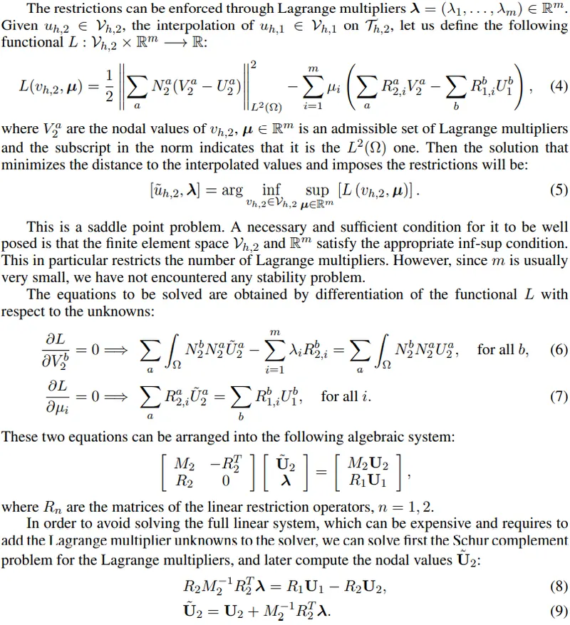
Note that system (8) is of small size m × m. The only difficulty for solving this problem is the calculation of M−1,2
. This is trivial if the mass matrix M2 is approximated by a diagonal matrix. If not, the problem can be solved using iterative methods, each iteration of which requires the solution of a system of equations with matrix M2; it is known that these systems can be solved with a small computational cost.
Non-linear restrictions
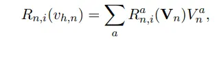
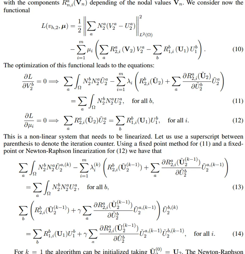
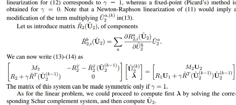
The same idea can be applied in the case in which the restrictions are non-linear, i.e., mappings Rn,i in (2) are non-linear. Let us assume that we write them as
Algebraic flux correction
The design philosophy of modern high-resolution schemes as presented by Zalesak [30] involves three main components which can be chosen and optimized individually:
1. an approximation to which they reduce in regions where the solution is smooth;
2. an approximation to which they reduce in the vicinity of shocks and steep fronts;
3. a mechanism for blending the above approximations at each node and time step so
as to satisfy the imposed physical or mathematical criteria.
In the preceding three sections, we specified the first two components and showed how to combine them within an iterative defect correction scheme. Now we can proceed to the design of flux limiters to be used for the computation of the correction factors αij in (19).
To this end, let us adopt a node-oriented limiting strategy which can be traced back to the flux-corrected transport (FCT) methodology [19],[28].
The limiting techniques to be considered are based on the following algorithm:
1. Compute the sums of positive/negative anti-diffusive fluxes into each node.
2. Select nodal correction factors so as to satisfy the algebraic constraints.
3. Check the sign of the anti-diffusive fluxes and limit them edge-by-edge.
Unlike many other algorithms, flux limiters of this form are fully multidimensional because they control the net anti-diffusive flux/solution increment rather than the slope ratio for a local three-point stencil or a similar smoothness indicator [16]. Below we discuss different options for the choice and enforcement of appropriate upper/lower bounds.
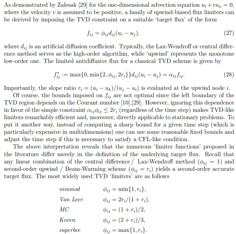
Upwind-biased flux limiting
Symmetric flux limiting
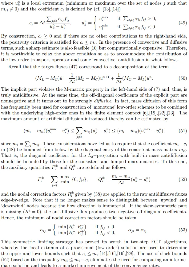
For genuinely time-dependent problems, mass lumping degrades the phase accuracy of finite element schemes and deprives them of significant advantage in comparison to finite difference and finite volume methods. Berzins [2],[3] recognized the need for including the consistent mass matrix in a positivity-preserving fashion and presented some ideas as to how this can be accomplished. As of this writing, no truly multidimensional extension of his methodology seems to be available, so we need to look for another way to embed the consistent mass matrix into algebraic flux correction schemes. In fact, our revised FEM-TVD algorithm (42)-(46) is applicable to target fluxes of the form (17). However, the upper/lower bounds may need to be redefined as explained below and the mass matrix contribution may be large enough to render the upwind-biased
limiting strategy impractical. As an alternative, we introduce asymmetric flux limiter which was largely inspired by the consistent-mass FEM-FCT algorithm [19],[20]. Let us start with a ‘stand-alone’ limiter for the mass anti-diffusion (ML − MC) ˙u such that
fij = mij ( ˙ui − u˙ j )

Combined flux limiting
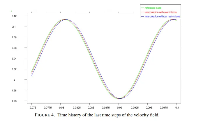
In light of the above, mass antidiffusion can be limited as if spatial differential operators were missing and vice versa. The symmetric limiting strategy (54)-(58) is appropriate for the former, while upwind-biased flux limiting of the form (42)-(46) lends itself to the treatment of the convective term. However, such an ‘operator splitting’ for the target flux (17) is undesirable because the independent limiting of its constituents (29) and (47) may produce an antidiffusive flux of greater magnitude than the original one. Indeed, the contribution of the consistent mass matrix and convective antidiffusion may have different signs. Our experience with flux correction of FCT type indicates that it is worthwhile to prelimit fij so as to prevent it from becoming diffusive and creating numerical artifacts [13],[16]. The corresponding coefficient φ T ij for the total flux (17) reads

References:
What’s The Difference Between FEM, FDM, and FVM? | Machine Design