Week 8 - Simulation of a backward facing step in OpenFOAM

AIM:-

in this challenge,you are going to simulate an in compressible-laminar-viscous floe through the

In this challenge you are going to simulate an in compressible-laminar-viscous flow through the backward facing step geometry. You should perform a transient simulation. The solver can be chosen based on the described physics of the flow. You need to explain the entire simulation procedure (how you set up the case).You should also provide explanations to every change you make inside the reference case files obtained from Open FOAM tutorials. You can choos the inlet velocity such that the flow is laminar.

After that ,you will perform 2 case studies as described below and compare the results.

Case 1- Simulation the flow without using any grading factor(i.r.,GF=1)

Case 2- Simulation the flow with grading factor of 0.2 The cells should be finer near the walls (including the step wall).

You can use the following mesh parameters but you can feel free to modify these values.

*Mesh specification

1. Number of cells along the x direction (longer dimension) =200

2.Number of cells along the loger y direction =20

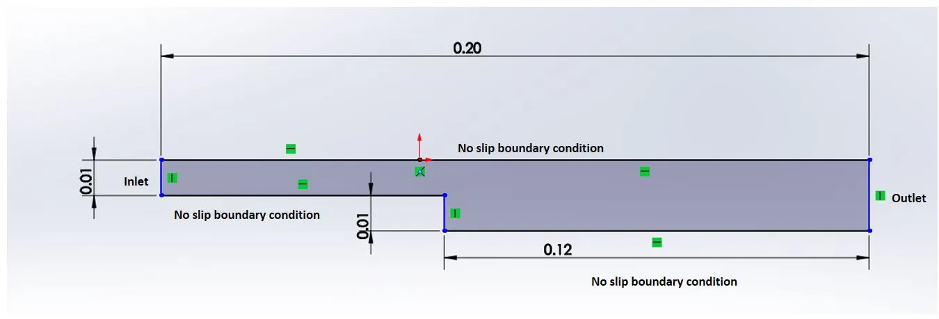
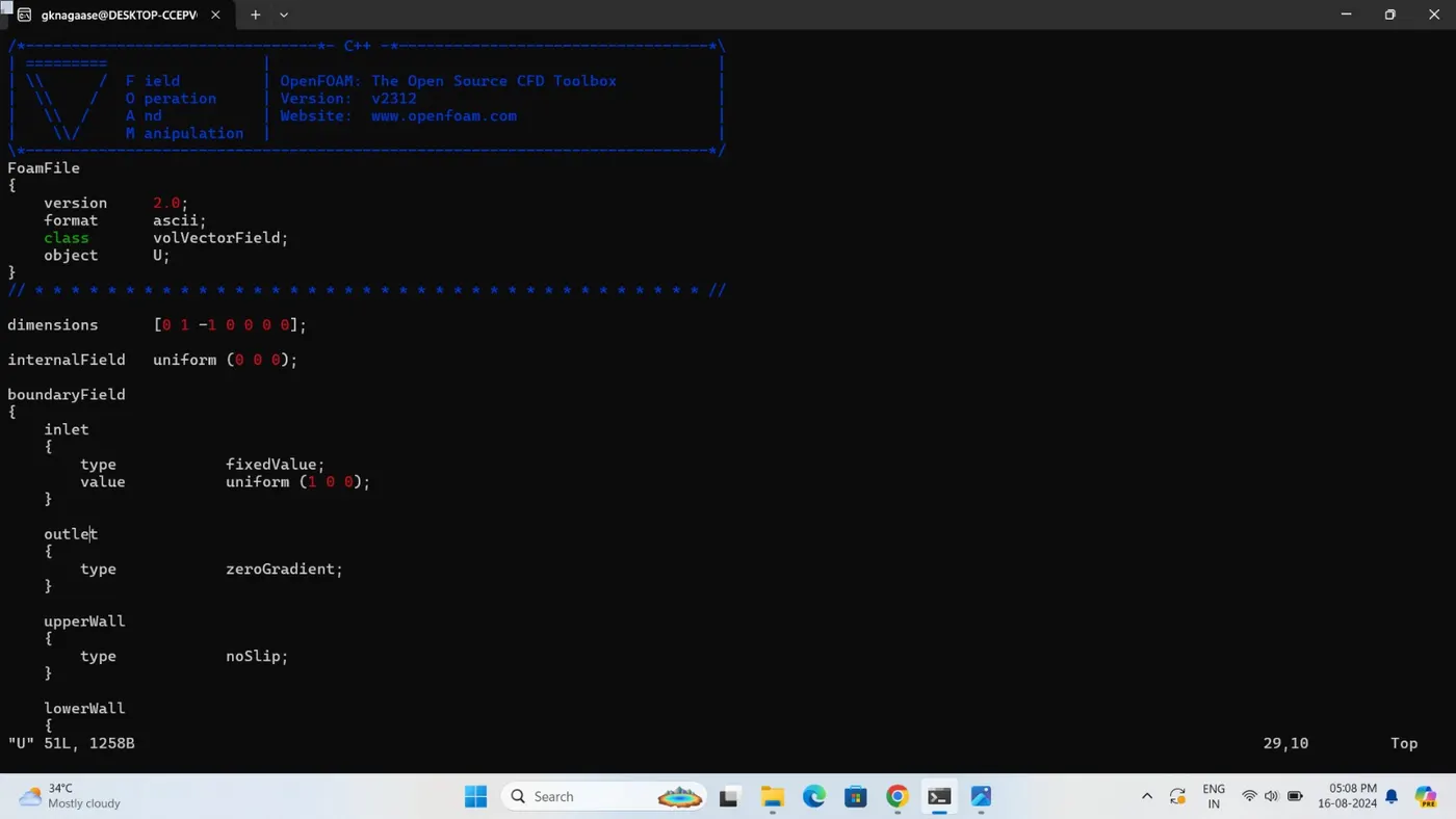
*Boundery condition specification

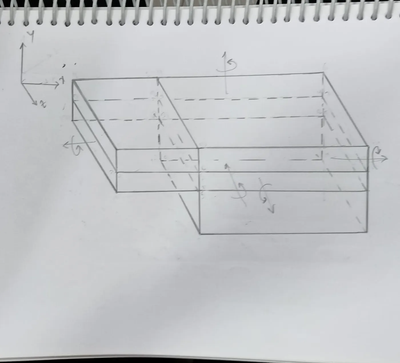
The domain specifications are provided in the following figure.

*Desired output

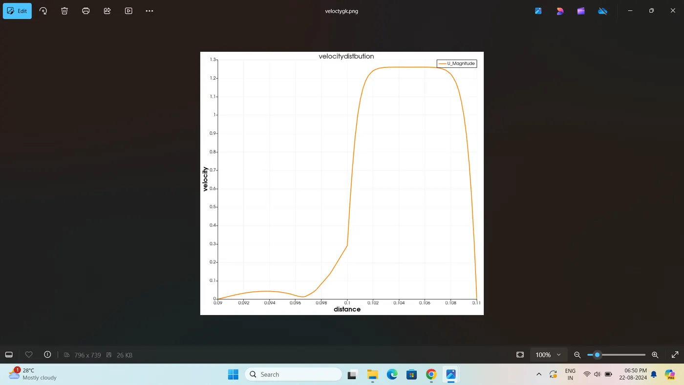
*Mesure the velocity profiie at 0.085 m from the geometry for both case studies and compaer .you can use the plot over line tool foe this

*Explain why Grading/Growth factor is essential for meshing.

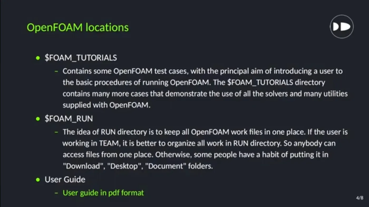
*Open Field Operation And Manipulation(FOAM)

*Open Foam operating systems steps

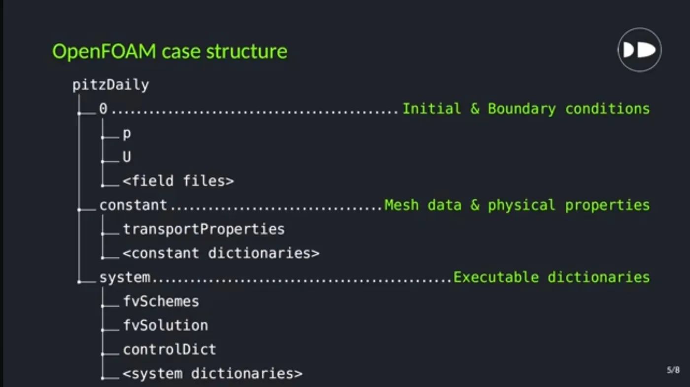
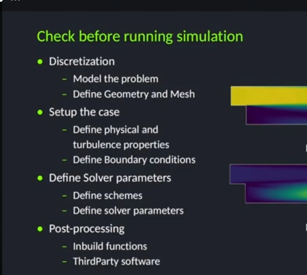
*Check before running simulation

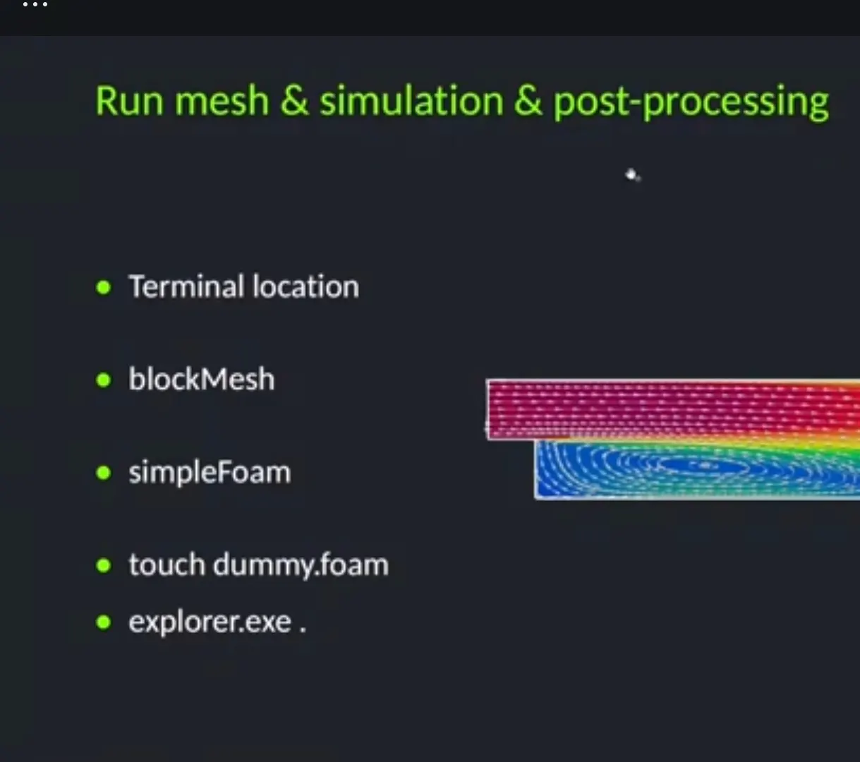
*Run mesh&simulation&post-processing

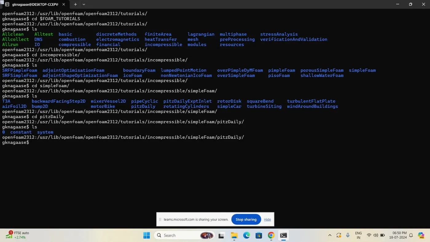
*Open foam opining

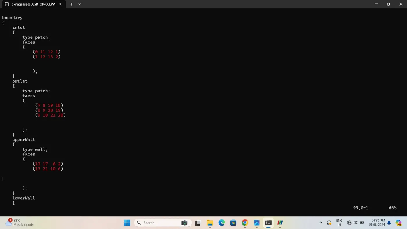
Vertices creating Diagram

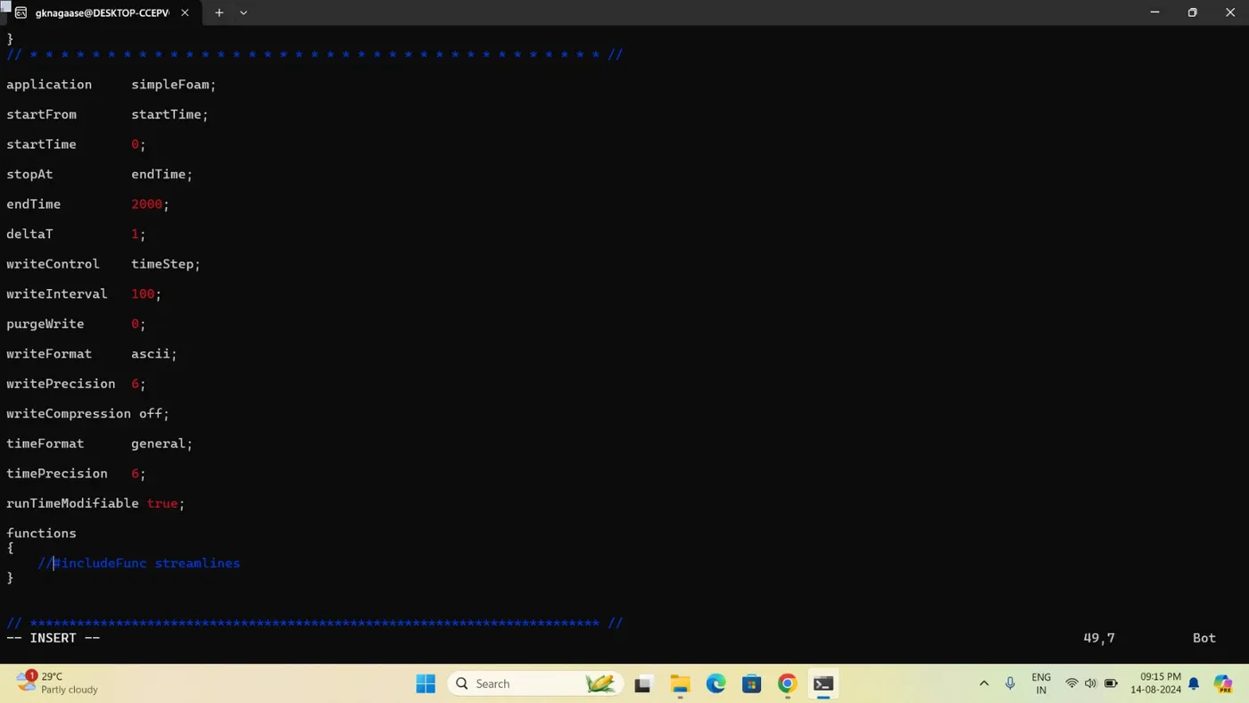
*Giving coding indicating

Backword-facing step

This tutorial will describe how to prepare-process,run and post-process a case involving isothermal,

In compressible flow across a backwards-facing step.

The problem is treated as two dimensional with the geometry shown in Figure

*an inlet opening(left);

*an outlet opening (right);

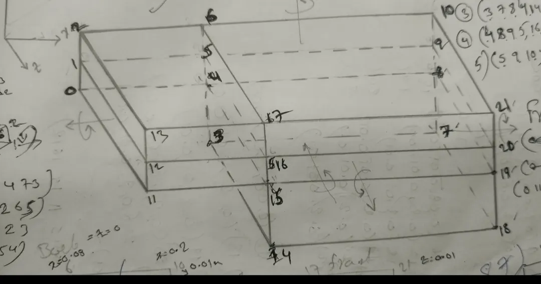
Entering open foam file

Pre-processing

Cases are configured in Open FOAM by editing input data files.Useres should selection a suitable file editor to do this e.g. Emacs vi,gedit,nedit,ect.

A case involves multiple data files,Corresponding to different parts of the configuration e.g.mesh,fields ,properties,control parameters,e.g.As described in section the set of files is stored within a case directory ,Which is given a suitable descriptive name.This tutorial uses the case $FOAM_TUTORIALS/incompressible..

Which this user should copy to their run directory as follows

cd $FOAM_RUN

CP -r $FOAM_TUTORIALS/modules/incompress

cd pitz Diaily Syteady

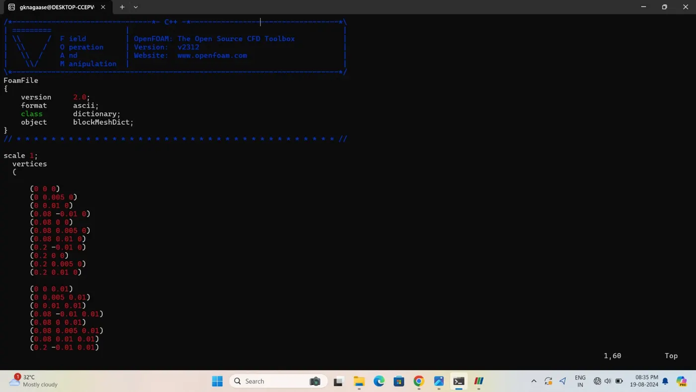
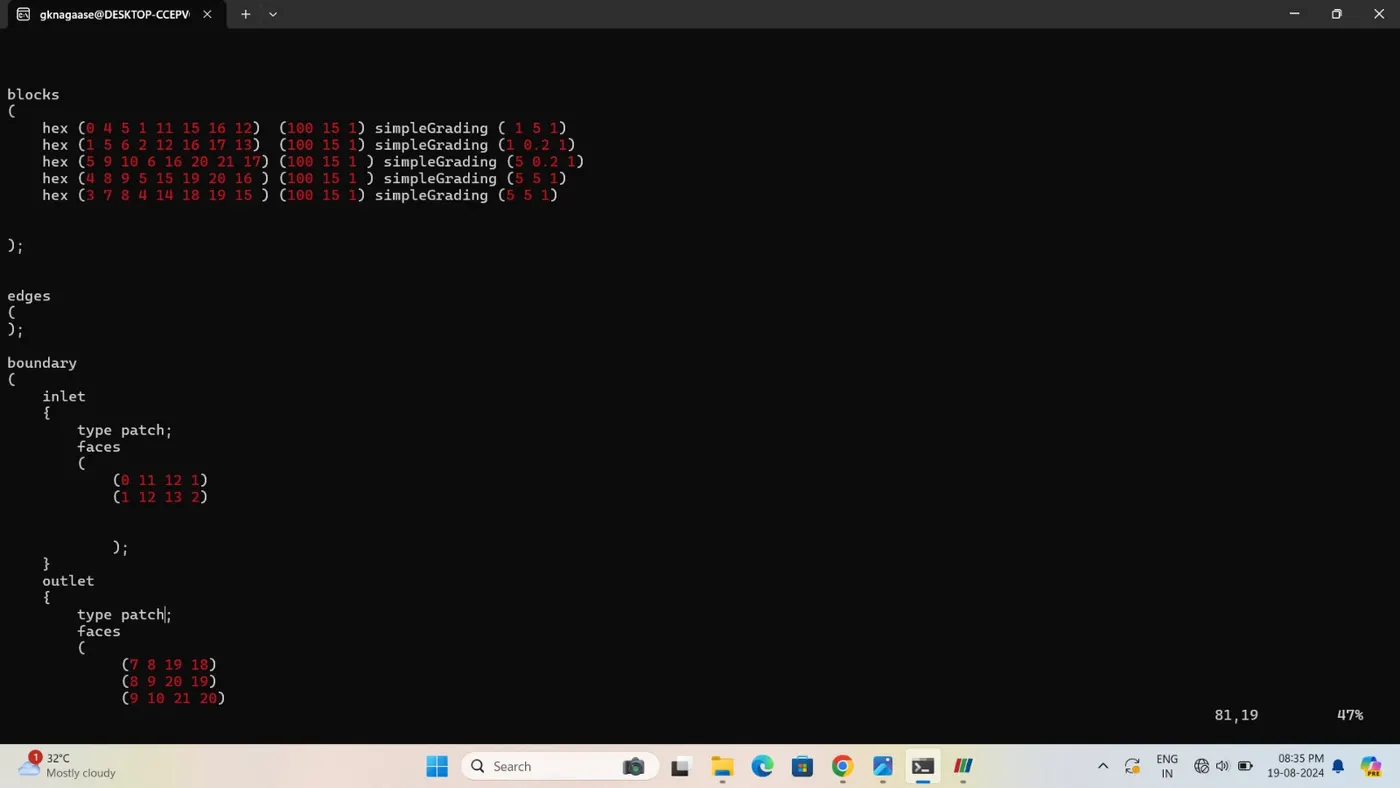
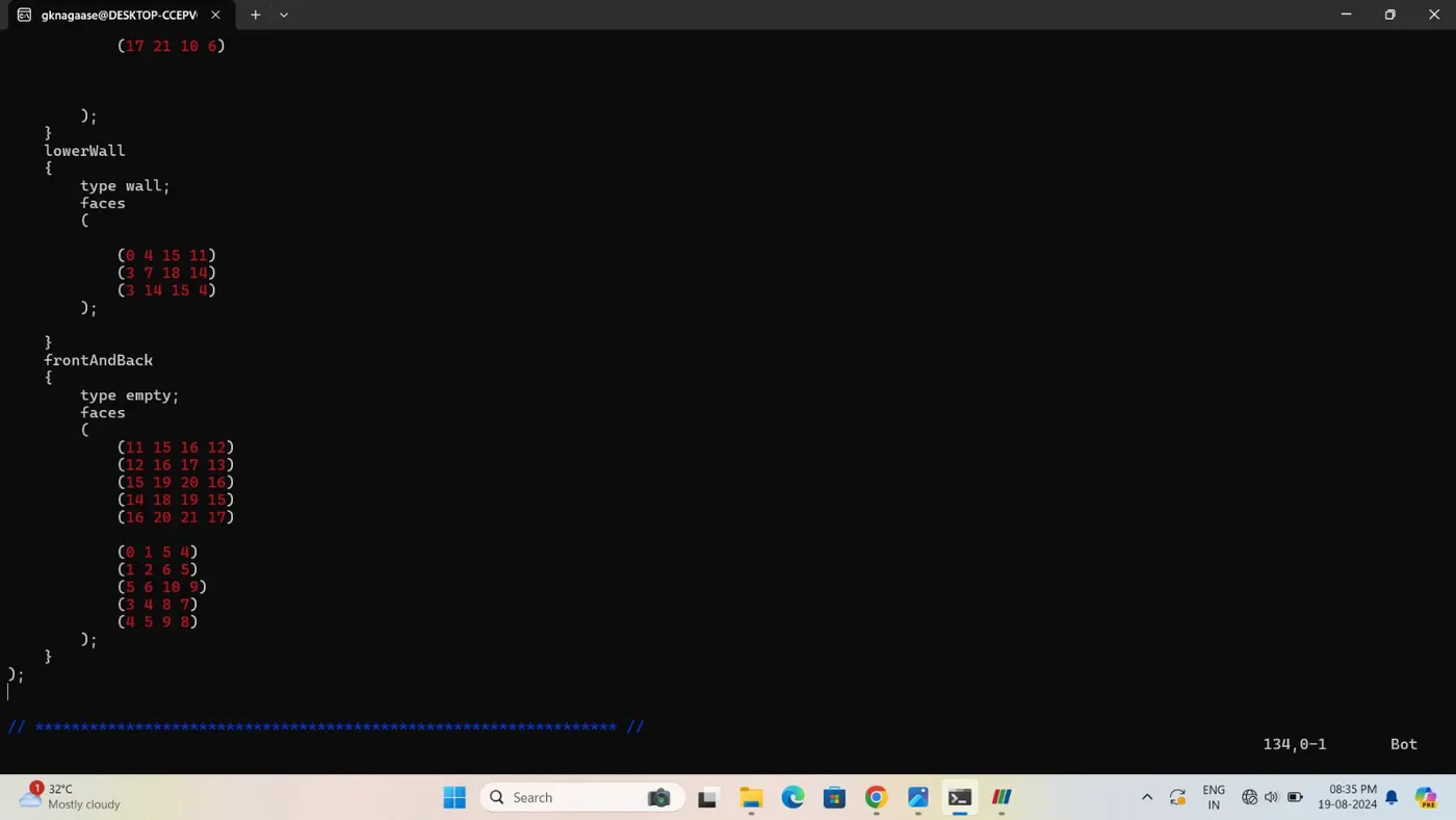
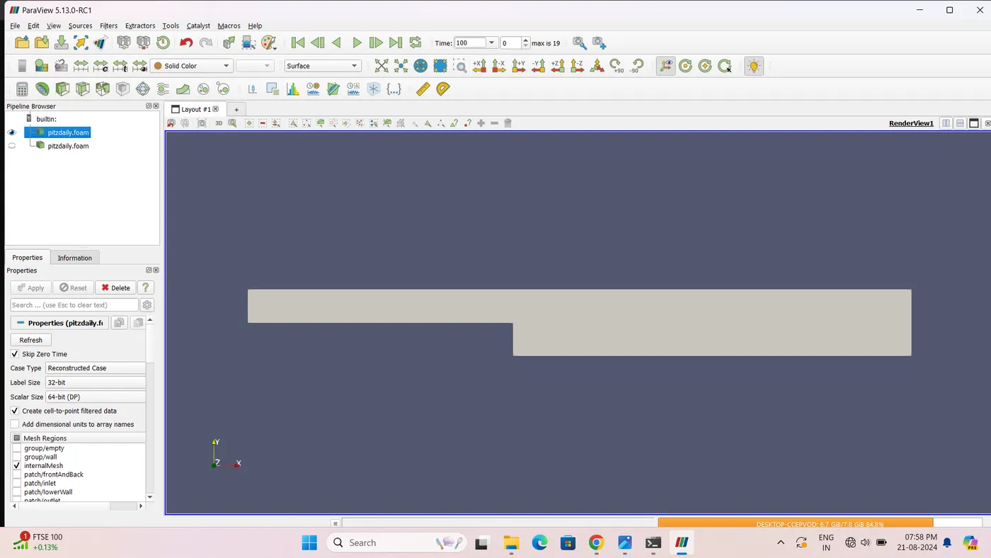
Meshing

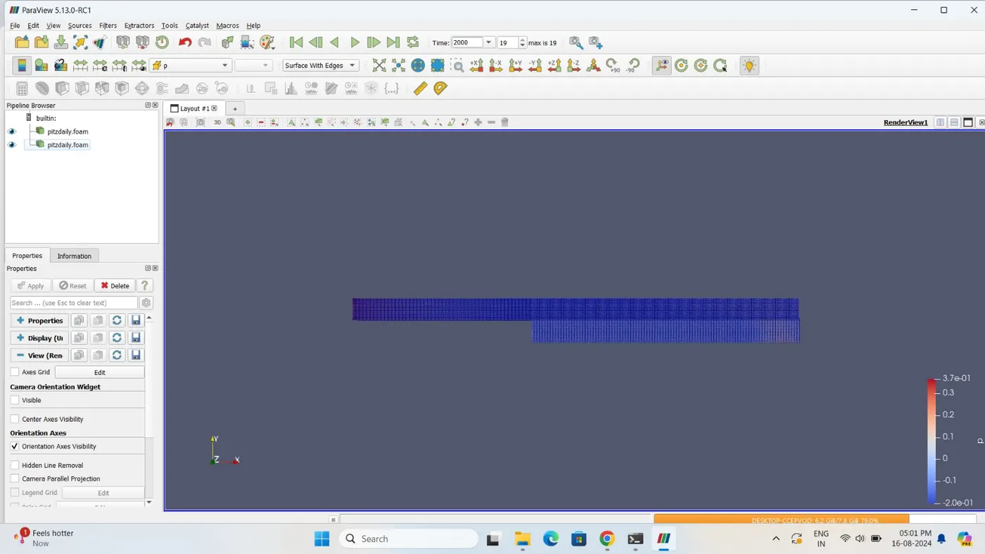
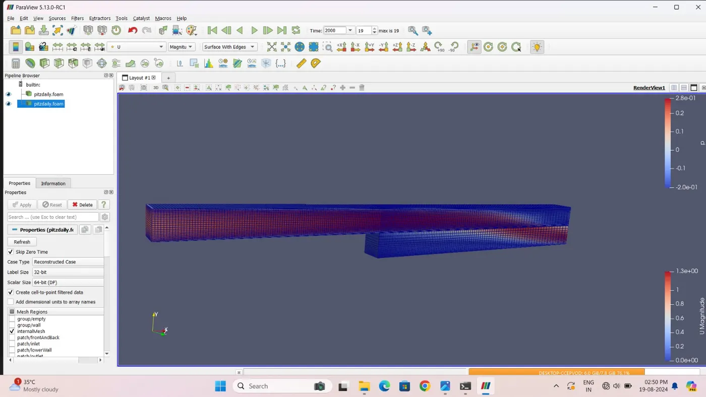
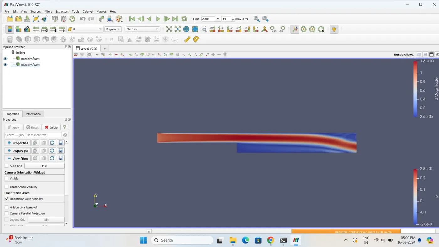
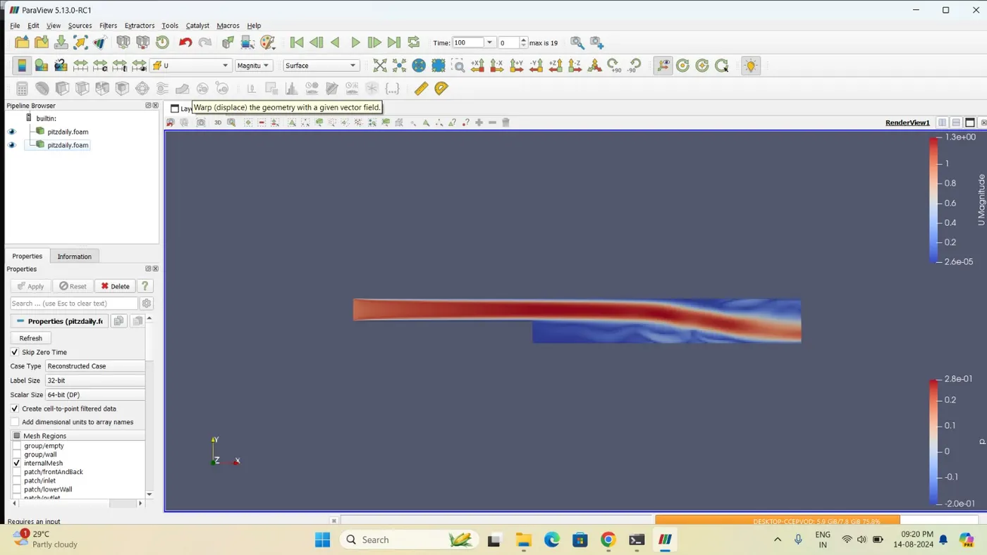
Vector plots

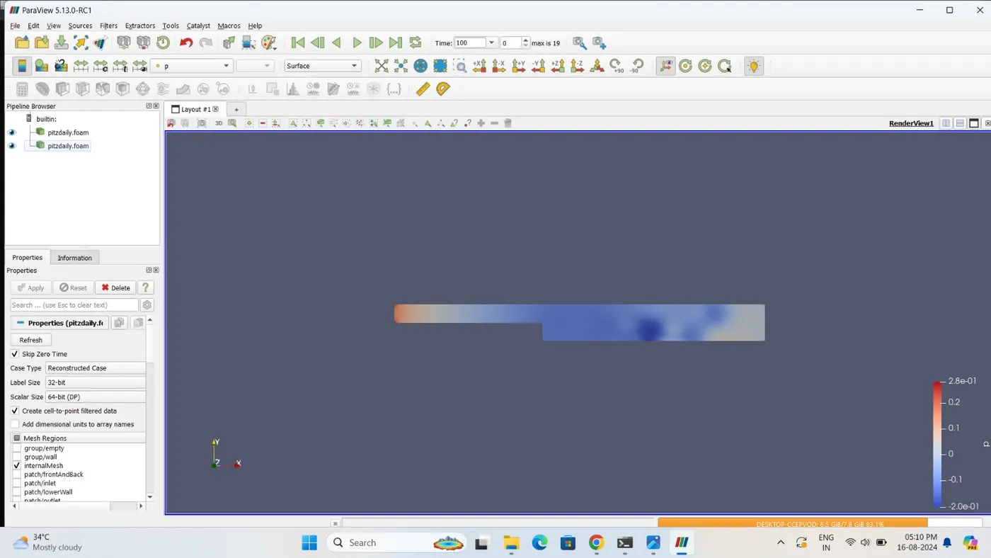
Before drawing vectors of the flow velocity, turn off the display of the Slice module by highlighting it in the Pipeline Browser and clicking the eye button to the left of it. The aim is to generate a vector glyph for velocity at the centre of each cell. We therefore first need to filter the cell centres from the mesh geometry as described in section 7.1.7. With the pitzDaily Steady. OpenFOAM module highlighted in the Pipeline Browser, the user should select Cell Centers from the Filters->Alphabetical menu and then click Apply.

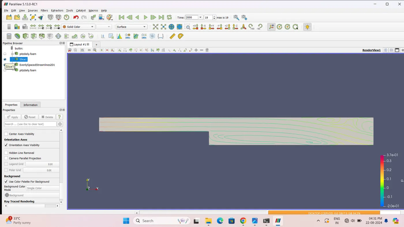
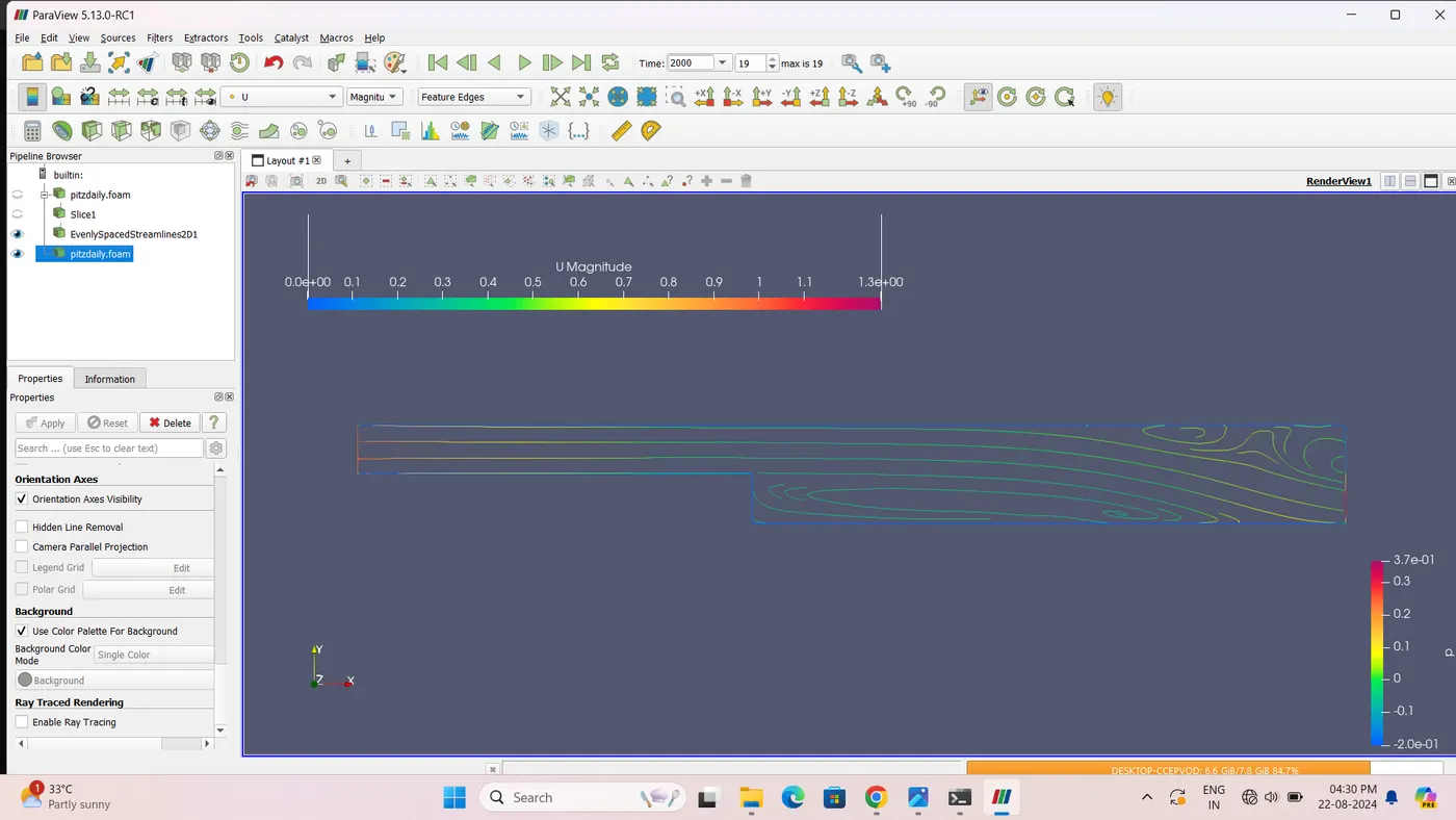
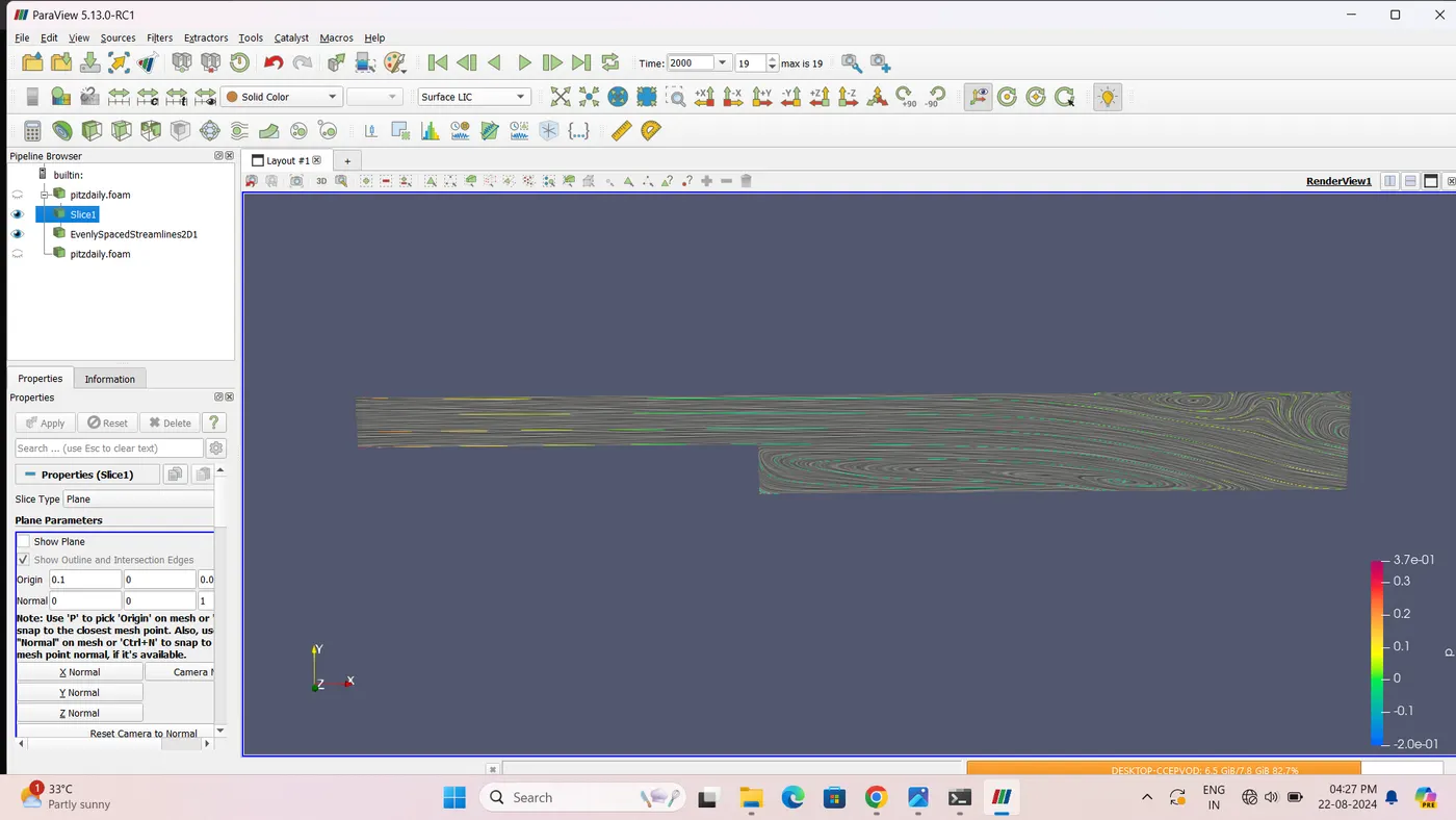
Contours

Before drawing contour lines of the flow speed, turn off the display of the Glyph module by highlighting it in the Pipeline Browser and clicking the eye button to its left. The user should then highlight the Slice module and colour by velocity U. We will then aim to draw contour lines on the slice at intervals of U of 1, 2, …, 10.

The contour lines can be drawn by applying the Contour filter to the slice. The filter draws lines in 2D, or surfaces in 3D, along constant values of scalar quantities. Contours cannot be drawn directly from U, since it is a vector, so we first need to generate a scalar field of the magnitude of U.

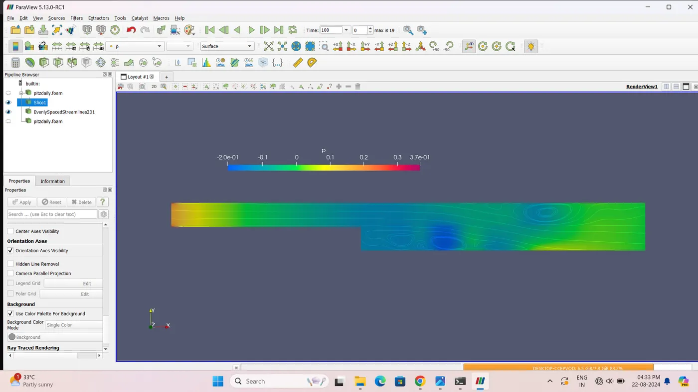
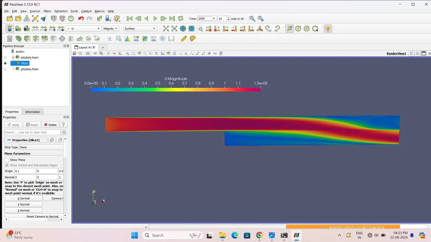
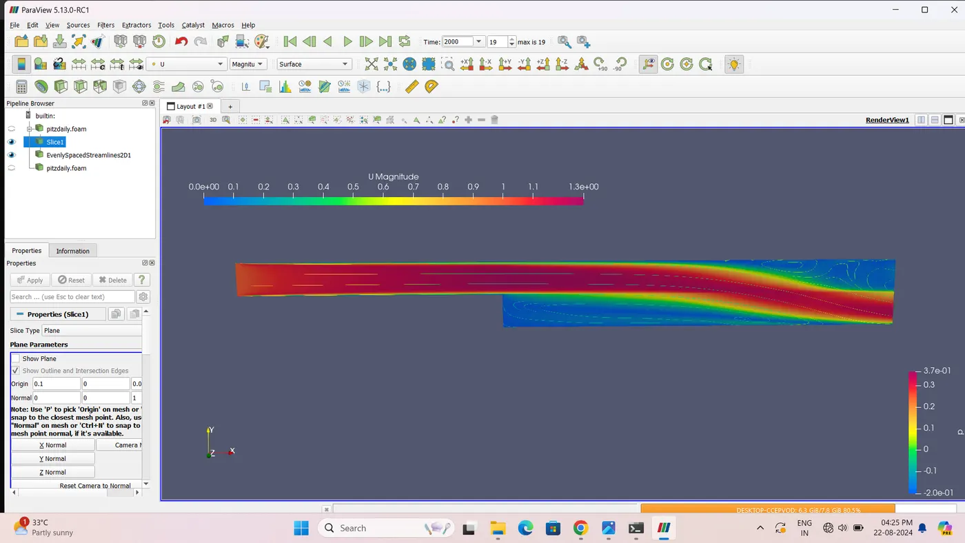
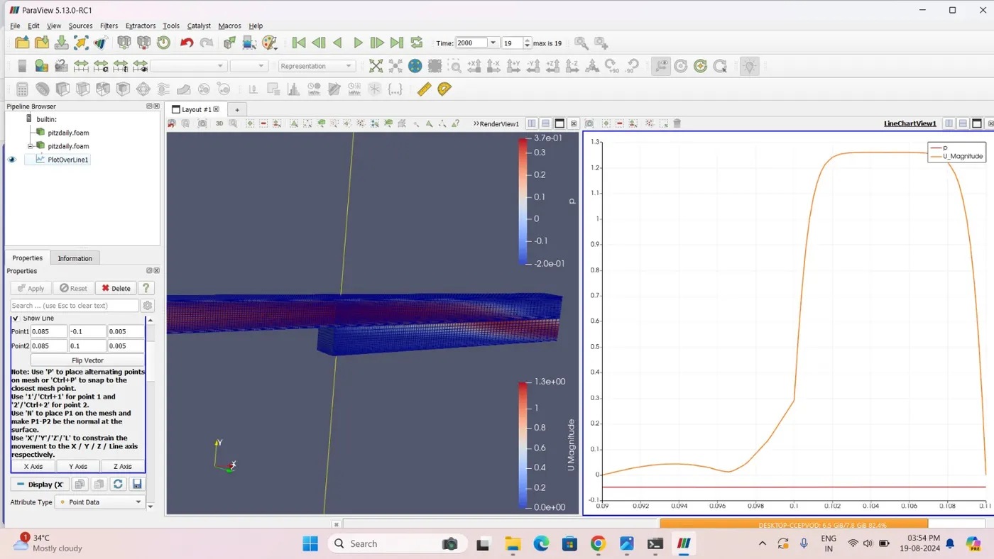
Velocity v/s Distance