Week 8 - Simulation of a backward facing step in OpenFOAM

Abstract: This study focus on the flow behavior of fluid through the Backward facing step using OpenFoam. And the results will be compared between two grading conditions.

Introduction:

Backward facing step: It is used to study the turbulence in internal flows. Sudden changes in geometry result in flow separation. This creates a zone of recirculation and a point of flow reattachment. Here we constructed the backward-facing step using blockMeshDict.

Flow: The flow considered here is an incompressible-laminar-viscous flow.

Solver: OpenFoam software was used for this study. IcoFoam is the relevant solver based on our flow assumption we can choose from OpenFoam. This solver uses Pressure-Implicit with splitting of operators ie PISO algorithm which is fast for solving laminar flow.

Preprocessing Mesh Model:

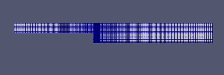
Geometry of the Backward facing step considered for study:

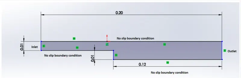
BlockMeshDict program generates the above geometry with normal grading:

/*--------------------------------*- C++ -*----------------------------------*\
  =========                 |
  \\      /  F ield         | OpenFOAM: The Open Source CFD Toolbox
   \\    /   O peration     | Website:  https://openfoam.org
    \\  /    A nd           | Version:  8
     \\/     M anipulation  |
\*---------------------------------------------------------------------------*/
FoamFile
{
    version     2.0;
    format      ascii;
    class       dictionary;
    object      blockMeshDict;
}
// * * * * * * * * * * * * * * * * * * * * * * * * * * * * * * * * * * * * * //

convertToMeters 1;

vertices
(
    (0 0 0)//0
    (0.08 0 0)//1
    (0.08 0.005 0)//2
    (0 0.005 0)//3
    (0.08 0.01 0)//4
    (0 0.01 0)//5  
    (0.2 0.01 0)//6
    (0.2 0.005 0)//7
    (0.2 0 0)//8
    (0.2 -0.01 0)//9
    (0.08 -0.01 0)//10
    (0 0 0.001)//11
    (0.08 0 0.001)//12
    (0.08 0.005 0.001)//13
    (0 0.005 0.001)//14
    (0.08 0.01 0.001)//15
    (0 0.01 0.001)//16
    (0.2 0.01 0.001)//17
    (0.2 0.005 0.001)//18
    (0.2 0 0.001)//19
    (0.2 -0.01 0.001)//20
    (0.08 -0.01 0.001)//21
);

blocks
(
    hex (0 1 2 3 11 12 13 14) (80 10 1) simpleGrading (1 1 1)
    hex (3 2 4 5 14 13 15 16) (80 10 1) simpleGrading (1 1 1)
    hex (2 7 6 4 13 18 17 15) (120 10 1) simpleGrading (1 1 1)
    hex (1 8 7 2 12 19 18 13) (120 10 1) simpleGrading (1 1 1)
    hex (10 9 8 1 21 20 19 12) (120 10 1) simpleGrading (1 1 1)
);

edges
(
);

boundary
(
    inlet
    {
        type wall;
        faces
        (
            (0 11 14 3)
            (3 14 16 5)
        );
    }
    outlet
    {
        type wall;
        faces
        (
            (9 8 19 20)
            (8 7 18 19)
            (7 6 17 18)
        );
    }
    frontAndBack
    {
        type empty;
        faces
        (
            (0 3 2 1)
            (3 5 4 2)
            (1 2 7 8)
            (2 4 6 7)
            (11 12 13 14)
            (14 13 15 16)
            (10 1 8 9)
            (12 13 18 19)
            (13 15 17 18)
            (21 12 19 20)
  

        );
    }
    noslipwalls
    {
        type wall;
        faces
        (
            (15 4 5 16)
            (17 6 4 15)
            (11 0 1 12)
            (21 10 9 20) 
            (1 10 21 12) 
        );
    }
        
);

mergePatchPairs
(
);

// ************************************************************************* //

Initial Conditions:

Pressure:

dimensions      [0 2 -2 0 0 0 0];

internalField   uniform 0;

boundaryField
{
    inlet
    {
        type            zeroGradient;
    }

    outlet
    {
        type            fixedValue;
        value           uniform 0;
    }

    frontAndBack
    {
        type            empty;
    }
    noslipwalls
    {
        type            zeroGradient;
    }
}

Velocity:

dimensions      [0 1 -1 0 0 0 0];

internalField   uniform (0 0 0);

boundaryField
{
    inlet
    {
        type            fixedValue;
        value           uniform (40 0 0);
    }

    outlet
    {
        type            zeroGradient;
    }

    frontAndBack
    {
        type            empty;
    }
    noslipwalls
    {
        type            noSlip;
    }
}

Timestep:

Run time: 0.2

time step size: 0.00001

Results:

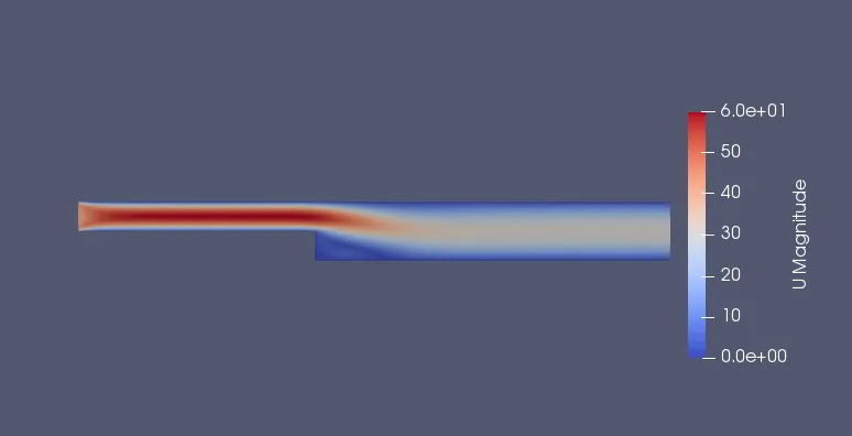
Case 1: Normal Grading of the mesh.

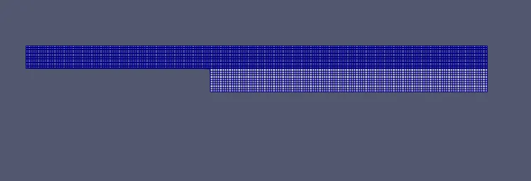
Velocity contour:

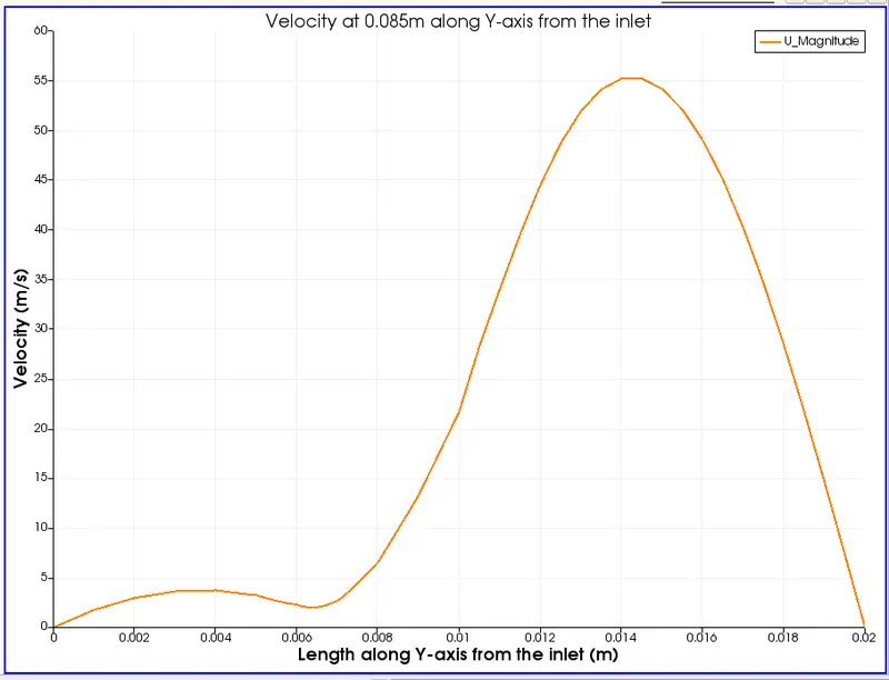
Velocity plot at 0.085m along Y-axis from the inlet:

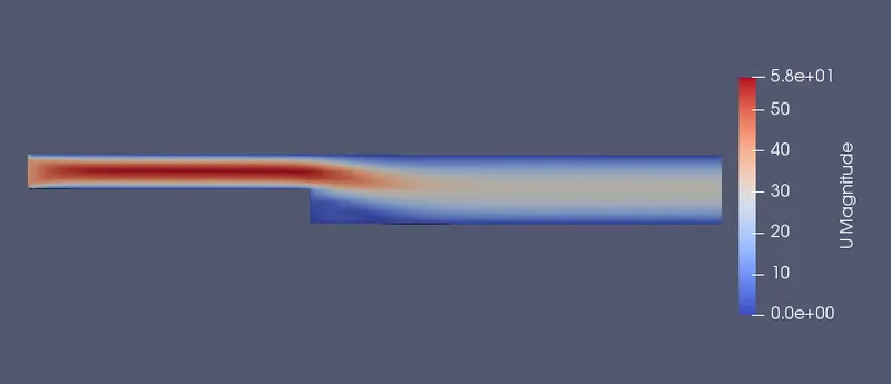
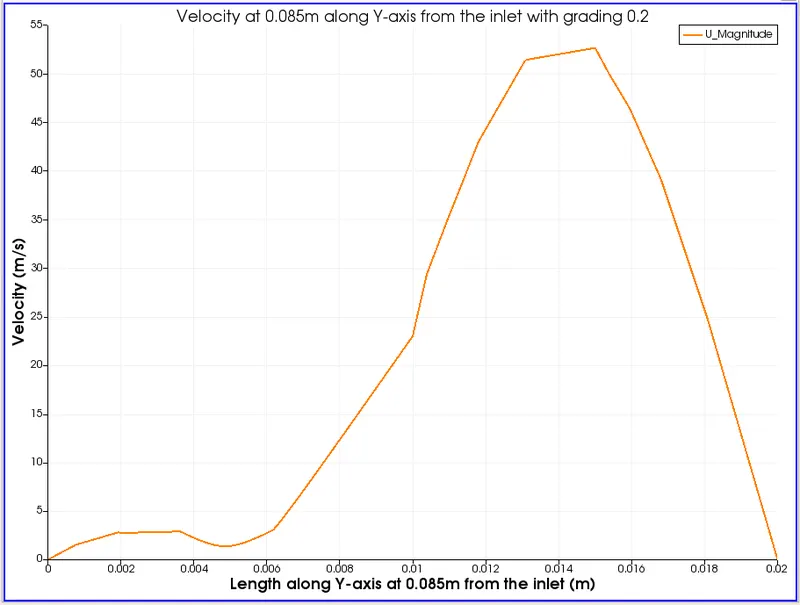
Case 2: Grading factor 0.2

Velocity contour:

Velocity plot:

Conclusion:

Here we simulated the incompressible laminar viscous flow through the backward-facing step using icoFoam solver from OpenFoam software. And generated the velocity plot along 0.085m from the inlet where the flow path gets expanded. By taking the velocity plots Case 1. without grading and Case 2. with grading factor 0.2 we can see a difference in the sharpness of the plots. Case 1 looks smooth in comparison with Case 2 because it doesn't have any grading. So Case 2 captures a more accurate velocity drop since we applied extra grading.

So by applying necessary mesh refinement in the critical areas we can get a more accurate plot.