Week 8 - Simulating Cyclone separator with Discrete Phase Modelling

• Aim:- To perform analysis on cyclone separator and calculate the separation efficiency and pressure drop.

• Objective:-

1. To write a few words about any four empirical models used to calculate the cyclone separator efficiency.
2. To perform an analysis on a given cyclone separator model by varying the particle diameter from 1 μm to 5 μm and calculate the separation efficiency in each case. Discuss the results. [Use both the velocity's as 3m/sec.]
3. To perform an analysis on a given cyclone separator model by varying the particle velocity from 1m/sec to 5 m/sec and calculate the separation efficiency and pressure drop in each case. Discuss the results. [Use particle diameter size as 5 μm for all cases & keep flow velocity same as particle velocity]

• Theory:-
• Cyclone Separator:- Cyclone separators are separation devices that use the principle of inertia to remove particulate matter from flue gases. Cyclone separator is one of many air pollution control devices known as pre-cleaners since they generally remove larger pieces of particulate matter. This prevents finer filtration methods from having to deal with large, more abrasive particles later on. In addition, several cyclone separators can operate in parallel, and this system is known as a multi-cyclone. It is important to note that cyclones can vary drastically in their size. The size of the cyclone depends largely on how much flue gas must be filtered, thus larger operations tend to need larger cyclones. For example, several different models of one cyclone type can exist, and the sizes can range from a relatively small 1.2-1.5 meters tall (about 4-5 feet) to around 9 meters (30 feet)—which is about as tall as a three-story building.

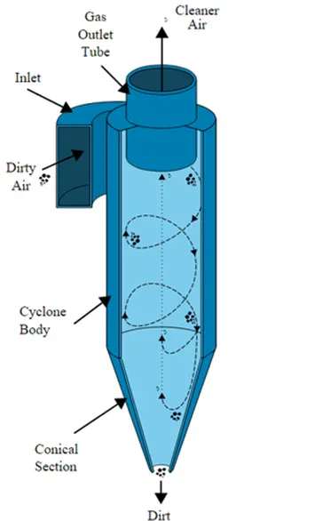
Working:- Cyclone separators work much like a centrifuge, but with a continuous feed of dirty air. In a cyclone separator, dirty flue gas is fed into a chamber. The inside of the chamber creates a spiral vortex, similar to a tornado. This spiral formation and the separation is shown in the Figure below. The lighter components of this gas have less inertia, so it is easier for them to be influenced by the vortex and travel up it. Contrarily, larger components of particulate matter have more inertia and are not as easily influenced by the vortex.

Most cyclones are built to control and remove particulate matter that is larger than 10 micrometers in diameter. However, there do exist high-efficiency cyclones that are designed to be effective on particles as small as 2.5 micrometers. As well, these separators are not effective on extremely large particulate matter. For particulates around 200 micrometers in size, gravity settling chambers or momentum separators are a better option.

Out of all of the particulate-control devices, cyclone separators are among the least expensive. They are often used as a pre-treatment before the flue gas enters more effective pollution control devices. Therefore, cyclone separators can be seen as "rough separators" before the flue gas reaches the fine filtration stages.

Effectiveness:- Cyclone separators are generally able to remove somewhere between 50-99% of all particulate matter in the flue gas. How well the cyclone separators are actually able to remove this matter depends largely on particle size. If there is a large amount of lighter particulate matter, less of these particles are able to be separated out. Because of this, cyclone separators work best on flue gases that contain large amounts of big particulate matter.

There are several advantages and disadvantages of using cyclone separators. First, cyclone separators are beneficial because they are not expensive to install or maintain, and they have no moving parts. This keeps maintenance and operating costs low. Second, the removed particulate matter is collected when dry, which makes it easier to dispose of. Finally, these units take up very little space. Although effective, there are also disadvantages in using cyclone separators. Mainly because the standard models are not able to collect particulate matter that is smaller than 10 micrometers effectively and the machines are unable to handle sticky or tacky materials well

• Empirical models used for cyclone separator efficiency:-

1. IOZIA AND LEITH MODEL:-

Iozia and Leith (1990) logistic model is a modified version of Barth (1956) model which is developed based on force balance. The model assumes that a particle carried by the vortex endures the influence of two forces: a centrifugal force Z, and flow resistance, W. Core length, zc, and core diameter dc, are given as

zc=(H−S)−H−S(DB)−1[(dcB)−1] for dc>B

zc=H−Szc=H−S for dc<Bdc<B

dc=0.47D(abD2)−0.25(DeD1.4)

The addition made by Iozia and Leith on the original Barth (1956) model is the core length zc and slope parameter β expression which is derived based on the statistical analysis of experimental data of cyclone with D = 0.25 m. The collection efficiency ηi of particle diameter dpi can be calculated from

ηi=11+(dpcdπ)β

where, dpc">dpcc=c0,at θ=0 is the 50% cut given by Barth (1956)

1. LI AND WANG MODEL:-

The Li and Wang (1989) model include particle bounce or re-entrainment and turbulent diffusion at the cyclone wall. A two-dimensional analytical expression of particle distribution in the cyclone is obtained. Li and Wang model was developed based on the following assumptions:

1. The radial particle velocity and the radial concentration profile are not constant, for uncollected particles within the cyclones.
2. Boundary conditions with the consideration of turbulent diffusion coefficient and particle bounce re-entrainment on the cyclone wall are:-

c=c0">r=D2

Dr∂c∂r=(1−α)wc at

The tangential velocity is related to the radius of cyclone by:-

uRn= constant

The concentration distribution in a cyclone is given as:-

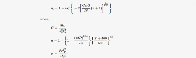
τi=ρpdpi218μ">Ne=1a(h+H−h2)

G is a factor related to the configuration of the cyclone, n is related to the vortex and τ is the relaxation term.

1. LAPPLE MODEL:-

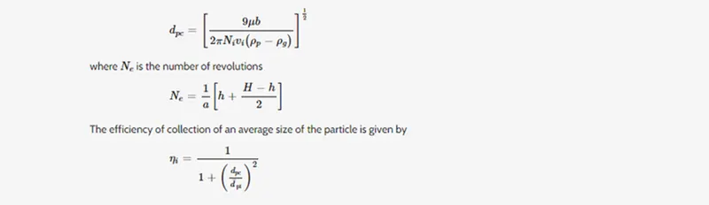
Lapple (1951) model was developed based on force balance without considering the flow resistance. Lapple assumed that a particle entering the cyclone is evenly distributed across the inlet opening. The particle that travels from inlet half-width to the wall in the cyclone is collected with 50% efficiency. The semi-empirical relationship developed by Lapple (1951) to
calculate a 50% cut diameter, dpc is

• Content:-

1. Geometry setup:-
2. Choose Fluid flow fluent and start with editing geometry.
3. Import the step file of the model into spaceclaim.

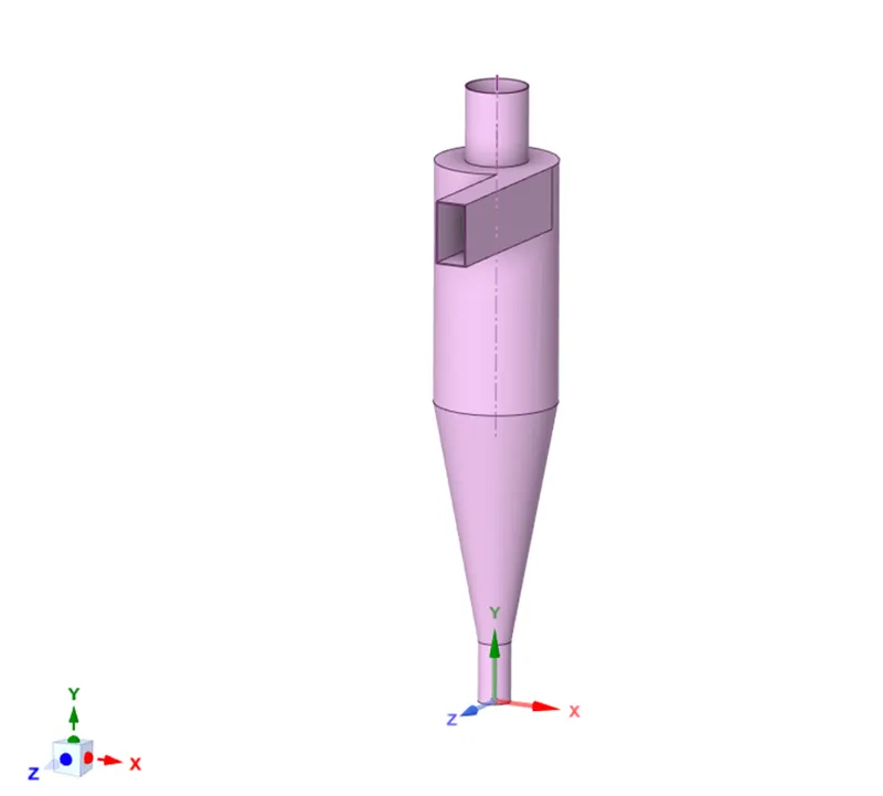
4.Volume extract the model so that we can analyse the fluid flow of the cyclone separator.

2) Meshing :-

• For meshing we open Meshing,where we mesh our model so that we can use it to solve our model.
• In general it is always good to name the surfaces before meshing. So let us do that.
• We first select the edges of inlet by using the edge selection so that we can provide name for our entity selection.

steps : select the inlet by using edge selection -> then press N -> name the selection as inlet.

• In the similar way we name the two outlets.
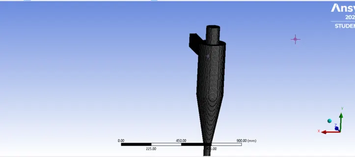
• Then next thing to do is to mesh.We click the mesh option in the side then give element size as 0.0053 mm .
• The below image is the final view of mesh .

• Now we have to check the quality of the mesh.

steps : mesh ->quality-> mesh metric-> Element quality

• Here our minimum quality is around 15 %,so we can move further for our solution setup.

3) Problem Setup :-

• To set up our problem we open Fluent and setup inital conditions , boundary conditions material etc.,
• We first start with checking the mesh quality using perform mesh check under domain.If no error is seen in console window then we can proceed further.
• Then we move move to setting up physics where we select the solver,viscous model etc.
• We use a steady state pressure based solver to solve our model.

Physics :-

General :-

Solver type : pressure based

time : steady state

velocity formulation : absolute

• We need to enable gravity by giving value for Y as -9.8 m/s^2 as gravity is acting in negative Y-direction.

models :-

viscous model : K-epsilon RNG model with standard wall functions

• K-epsilon RNG model is a slight modification of the standard k-epsilon which ehances the accuracy of swirl dominated flows. Here we have to select swirl dominated flow.

Material :-

Fluid : Air

Discrete Phase Modelling (DPM) setup :-

• There are two ways of modelling DPM :-

1. One way Coupling:-
   The fluid phase influences the discrete phase via drag and turbulence.
   The discrete phase has no influence on the continuous phase.
2. Two-way coupling:-
   The continuous phase influences the discrete phase via drag and turbulence.
   The discrete phase influences the continuous phase via source terms of mass, momentum, and energy.
   It alternately solves the discrete and continuous phase equations until the solutions in both phases stop changing.

• Since here size of the particle we inject in the cyclone seperator is very small ,usage of both the type of flow shouldn't matter much. Here we select the interaction with continous phase to enable two way coupled flow .
• Update DPM sources every flow iteration ,enabling this option will give you the option of calculating the particle source term at every iteration.We will enable it.
• DPM iteration interval , this option will allows you to control the frequency at which the particles are tracked.We go with default value of 10 itself.

Tracking Parameters:-

We need to use two parameters to control the time integration of the particle trajectory equations:

1.Maximum number of steps :-

This factor is used to abort trajectory calculations when the particle never exits the flow domain and reports the trajectory fate as "incomplete''. The limit on the number of integration time steps eliminates the possibility of a particle being caught in a recirculating region of the continuous phase flow field and being tracked infinitely. The maximum number of steps can be increased up to a limit of 10e9 as per application.Here we give a value of 500000.

2. Length Scale, L :-

• Length scale controls the integration time step size used to integrate the equations of motion for the particle. The integration time step(Δt) is computed by ANSYS FLUENT based on a specified length scale L, and the velocity of the particle u_p and of the continuous phase u_c.
• L is proportional to the integration time step and is equivalent to the distance that the particle will travel before its motion equations are solved again and its trajectory is updated. A smaller value for the Length Scale increases the accuracy of the trajectory and heat/mass transfer calculations for the discrete phase.

(Note that particle positions are always computed when particles enter/leave a cell; even if you specify a very large length scale, the time step used for integration will be such that the cell is traversed in one step.

3. Step length Factor :-

• Step Length Factor also controls the time step size used to integrate the equations of motion for the particle. It differs from the Length Scale in that it allows ANSYS FLUENT to compute the time step in terms of the number of time steps required for a particle to traverse a computational cell. To set this parameter instead of the Length Scale, turn off the Specify Length Scale option.
• The integration time step is computed by ANSYS FLUENT based on a characteristic time that is related to an estimate of the time required for the particle to traverse the current continuous phase control volume. If this estimated transit time is defined as Δt^*, ANSYS FLUENT chooses a time step Δt as,
• Where λ is the Step Length Factor. λ is inversely proportional to the integration time step and is roughly equivalent to the number of time steps required to traverse the current continuous phase control volume. A larger value for the Step Length Factor decreases the discrete phase integration time step.
• One simple rule of thumb to follow when setting the parameters above is that if you want the particles to advance through a domain consisting of N mesh cells into the main flow direction, the Step Length Factor times N should be approximately equal to the Max. Number of Steps.
• We can give any one as a input.So here we keep the default value for Step Length Factor i.e., 5.

Injections :-

• Now we have to specifty the injections of the discrete particles on to the continuous phase.So to do this we have to open injections in the discrete phase modelling.
• click on injections -> then create

Particle type : Inert

Material : Anthracite

Injection type : Surface injection

Release from surface : Inlet

• In the bottom enable inject using face normal direction
• Then in the point properties -> then in that give following values for each variable .

Diameter : 1e-6 m

Velocity magnitude : 3 m/sec

Total flow rate : 1e-20 kg/sec

• Then click ok and close discrete phase modelling.

Boundary conditions :-

Inlet - Velocity inlet

velocity : 3 m/sec

DPM : reflect

Outlet (Top) - Pressure outlet

Gauge pressure : 0 pa

DPM : Escape

Outlet(Bottom) - Pressure outlet

Gauge pressure : 0 pa

DPM : Trap

• Then we have to initialize, then we do Standard initialization from inlet .
• Then in solution method for Pressure velocity coupling SIMPLE scheme is used.

4) Solving :-

• Then we are ready to solve .We run the simulation by giving no. of iterations = 1000.
• Then export the particle tracking data for that,

File -> export->particle history data -> select injection -> then give name and place to save for that file by selecting browse -> Then click on write.

• Then in console you can see number of particles data where you will find total number of particles as 372 .Then let us post process the results.

5)Post processing :-

• Then open CFD post and import the results for that,

Open results -> Import the data by selecting file -> then select import -> thenselect import fluent particle track file -> Then open saved file .

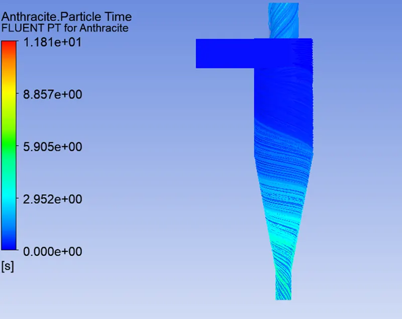
• Then you can see fluent PT for anthracite file after import .Then double click on that you can give maximum number of particles to display ,as we have tracked 372 particles let us give 372.
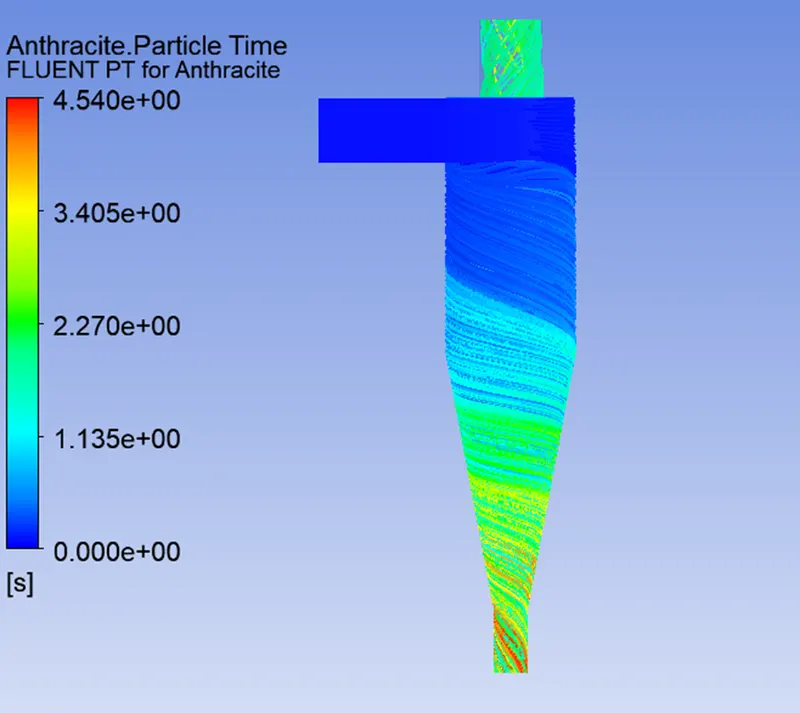
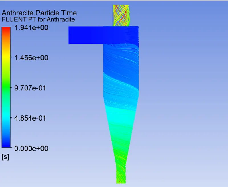
• Then let us colour particle track by the anthracite particle time, which shows the residence time of each particle.

Anthracite particle time contour :-

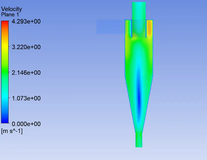
Velocity contour :-

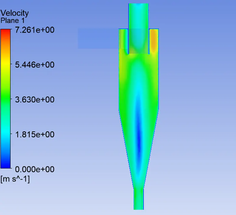
• In the below image we can see the velocity contour on the midplane of cyclone separator .

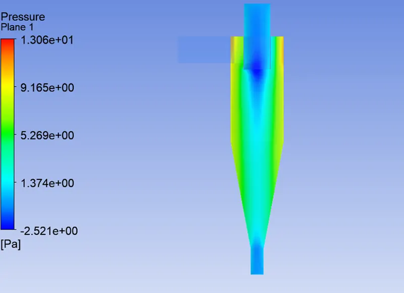
Pressure contour :-

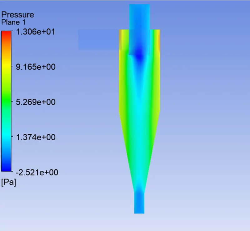
• In the below image we can see the pressure contour on the midplane of cyclone separator .

Residuals plot :-

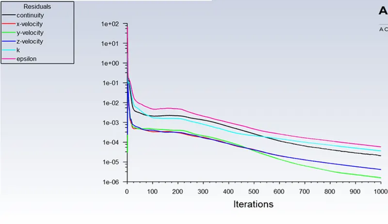
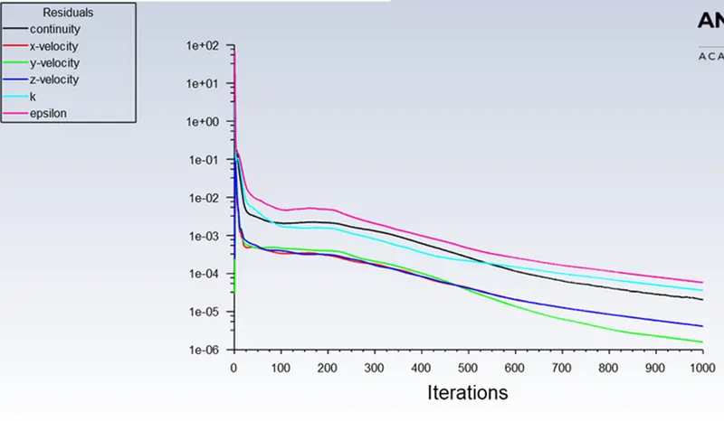
• You can observe from the below plot the residuals has converged.

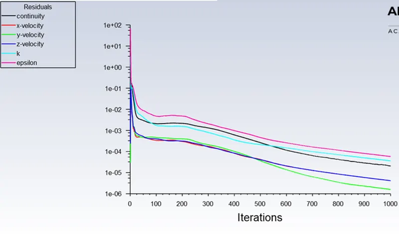
Case -2 :- particle diameter of 3 μm :

• Everything is same as previous case from the point of geometry and mesh.
• Comming to set up the only change here is in the injections in the discrete phase modelling we give particle dia meter as 3 μm .Remaining everything is same as previous case.
• Then we run for 1000 iterations .
• So let us directly run the simulation and then post process the results.

Post processing :-

• Then open CFD post and import the results for that,

Open results -> Import the data by selecting file -> then select import -> then select import fluent particle track file -> Then open newly saved file .

• Then you can see fluent PT for anthracite file after import .Then double click on that you can give maximum number of particles to display ,as we have tracked 372 particles let us give 372.
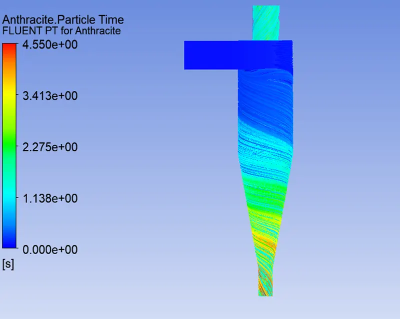
• Then let us colour particle track by the anthracite particle time, which shows the residence time of each particle.

Anthracite particle time contour :-

Velocity contour :-

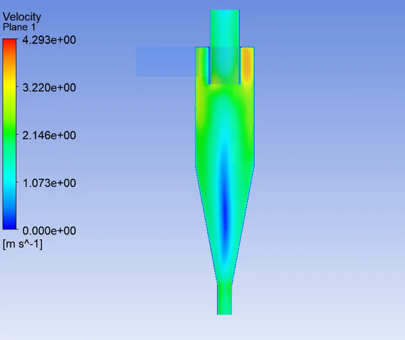
• In the below image we can see the velocity contour on the midplane of cyclone separator .

Pressure contour :-

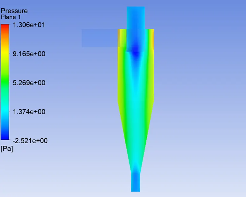
• In the below image we can see the pressure contour on the midplane of cyclone separator .

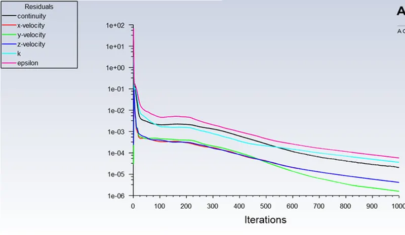
Residuals plot :

• You can observe from the below plot the residuals has converged.

Case -3 :- particle diameter of 5 μm :-

• Everything is same as previous case from the point of geometry and mesh.
• Comming to set up the only change here is in the injections in the discrete phase modelling we give particle dia meter as 5 μm .Remaining everything is same as previous case.
• Then we run for 1000 iterations .
• So let us directly run the simulation and then post process the results.

Post processing :-

• Then open CFD post and import the results for that

Open results -> Import the data by selecting file -> then select import -> then select import fluent particle track file -> Then open newly saved file .

• Then you can see fluent PT for anthracite file after import .Then double click on that you can give maximum number of particles to display ,as we have tracked 372 particles let us give 372.
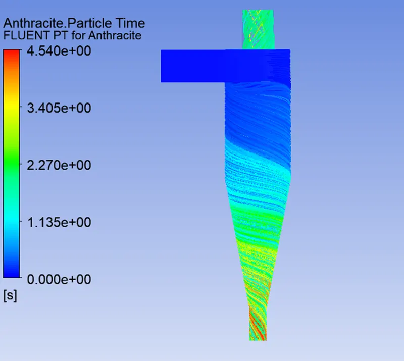
• Then let us colour particle track by the anthracite particle time, which shows the residence time of each particle.

Anthracite particle time contour :-

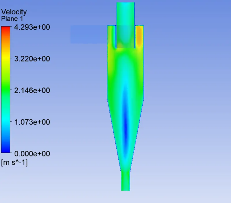
Velocity contour :

• In the below image we can see the velocity contour on the midplane of cyclone separator .

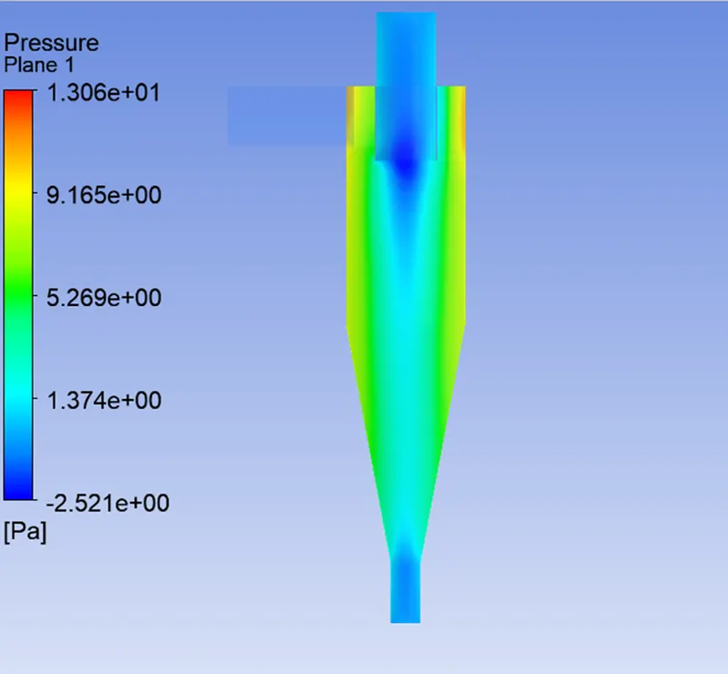
Pressure contour :-

• In the below image we can see the pressure contour on the midplane of cyclone separator .

Residuals plot :-

• You can observe from the below plot the residuals has converged.

Conclusions :-

• Here let us tabulate all the results of all the cases and discuss the results of the simulation.

Performing an analysis on cyclone separator model by by varying the particle velocity from 1 m/sec to 5 m/sec :-

• Here we perform an analysis on a given cyclone separator model by varying the particle velocity from 1 m/sec to 5 m/sec and calculate the separation efficiency and pressure drop in each case.Then we discuss the results.Here we use particle diameter size as 5 μm for all cases & keep flow velocity same as particle velocity.
• Let us perform the simulation for each case by following the above procedure.

Case -1 :- particle velocity of 1 m/sec :-

• Everything is same as previous case from the point of geometry and mesh.
• Comming to set up the changes here is in the injections in the discrete phase modelling we give particle dia meter as 5 μm and here we keep flow velocity same as particle velocity = 1 m/sec remaining everything is same as previous case.
• Then we run for 1000 iterations .
• So let us directly run the simulation and then post process the results.

Post processing :-

• Then open CFD post and import the results for that,

Open results -> Import the data by selecting file -> then select import -> then select import fluent particle track file -> Then open newly saved file .

• Then you can see fluent PT for anthracite file after import .Then double click on that you can give maximum number of particles to display ,as we have tracked 372 particles let us give 372.
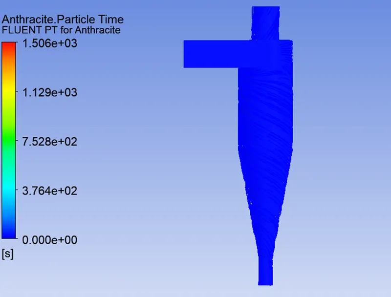
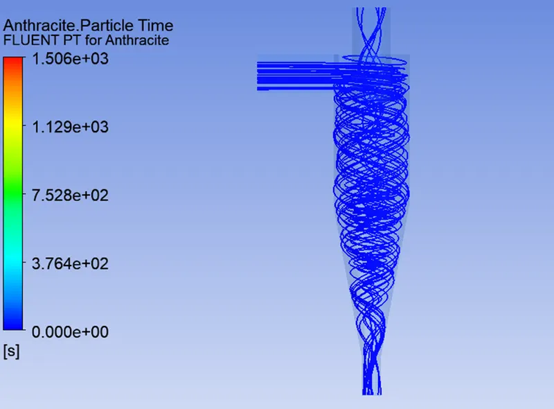
• Then let us colour particle track by the anthracite particle time, which shows the residence time of each particle.

Anthracite particle time contour :-

Anthracite particle time contour for 372 particles

• For better visualization of anthracite particle time contour , let us give particle count as 25 particles.

Velocity contour :-

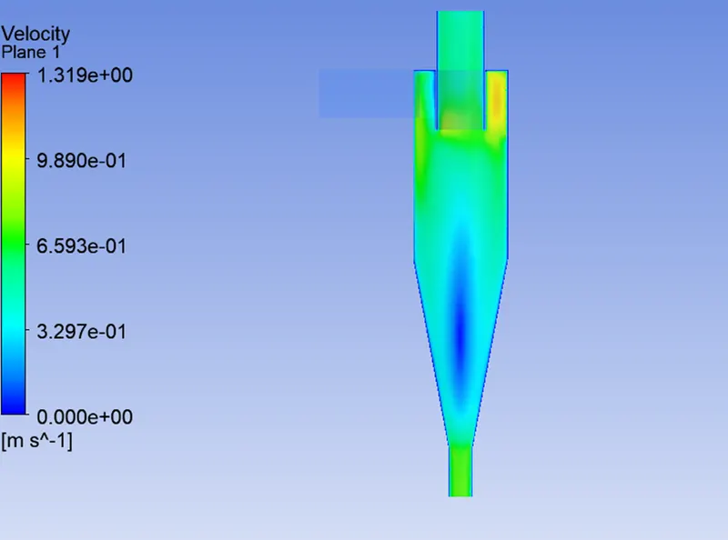
• In the below image we can see the velocity contour on the midplane of cyclone separator .

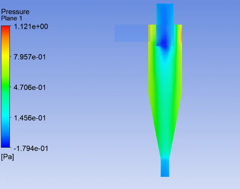
Pressure contour :-

• In the below image we can see the pressure contour on the midplane of cyclone separator .

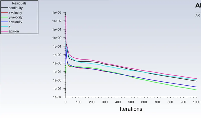
Residuals plot :-

• You can observe from the below plot the residuals has converged.

Case -2 :- particle velocity of 3 m/sec :-

• Everything is same as previous case from the point of geometry and mesh.
• Comming to set up the changes here is in the injections in the discrete phase modelling we give particle diameter as 5 μm and here we keep flow velocity same as particle velocity = 3 m/sec remaining everything is same as previous case.
• Then we run for 1000 iterations .
• So let us directly run the simulation and then post process the results.

Post processing :-

• Then open CFD post and import the results for that,

Open results -> Import the data by selecting file -> then select import -> then select import fluent particle track file -> Then open newly saved file .

• Then you can see fluent PT for anthracite file after import .Then double click on that you can give maximum number of particles to display ,as we have tracked 372 particles let us give 372.
• Then let us colour particle track by the anthracite particle time, which shows the residence time of each particle.

Anthracite particle time contour :-

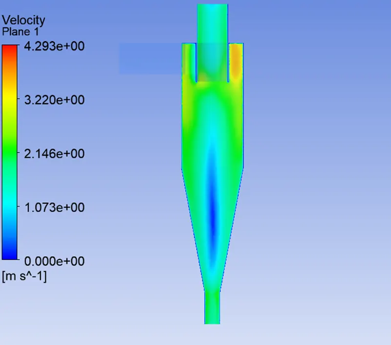
Velocity contour :-

• In the below image we can see the velocity contour on the midplane of cyclone separator .

Pressure contour :-

• In the below image we can see the pressure contour on the midplane of cyclone separator .

Residuals plot :-

• You can observe from the below plot the residuals has converged.

Case -3 :- particle velocity of 5 m/sec :-

• Everything is same as previous case from the point of geometry and mesh.
• Comming to set up the changes here is in the injections in the discrete phase modelling we give particle diameter as 5 μm and here we keep flow velocity same as particle velocity = 5 m/sec remaining everything is same as previous case.
• Then we run for 1000 iterations .
• So let us directly run the simulation and then post process the results.

Post processing :-

• Then open CFD post and import the results for that,

Open results -> Import the data by selecting file -> then select import -> then select import fluent particle track file -> Then open newly saved file .

• Then you can see fluent PT for anthracite file after import .Then double click on that you can give maximum number of particles to display ,as we have tracked 372 particles let us give 372.
• Then let us colour particle track by the anthracite particle time, which shows the residence time of each particle.

Anthracite particle time contour :-

Velocity contour :-

• In the below image we can see the velocity contour on the midplane of cyclone separator .

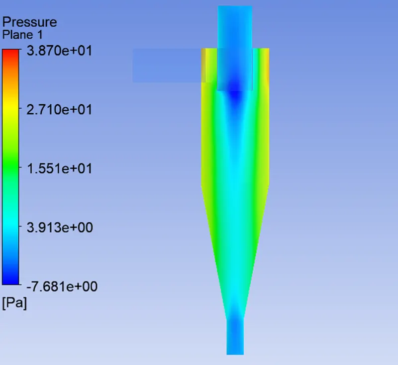
Pressure contour :-

• In the below image we can see the pressure contour on the midplane of cyclone separator .

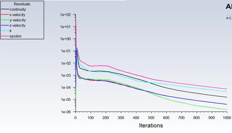
Residuals plot :-

• You can observe from the below plot the residuals has converged.

Conclusions :-

• Here let us conclude by comparing the results between all the cases and discuss the results of the simulation.
• In the above table you can observe that as the particle velocity increasing ,you can observe that number of particles trapped at the bottom outlet increasing which also increases the separation efficiency of the cyclone separator.
• When the velocity of the particle and diameter of the particle are very small,you can see a lot of incomplete particles leading to low separation efficiency.
• As the flow and particle velocity are increasing the pressure drop across the cyclone separator also increasing.
• They are actually built to control or remove particle matter that are larger than 10 μm.But a high efficiency cyclone seperator can filter out particles that are as small as 2.5μm.Altough these devices are inexpensive they are however not very effective when larger particular matter around the size of 200 μm come into play.In these cases devices such as gravity settling chamber or momentum separators are better option.