Week 8 - Simulating Cyclone separator with Discrete Phase Modelling
AIM: to simulate the flow through a cyclone separator and showing the results for the different particle size and for the different velocities.
we have to run the simulation for the six cases
1).set the velocity constant to 3 m/s and do simulation for the varying size of the particle.
2).set the particle size to constant and simulate for the different velocities.
models of the cyclone separator:
Cyclone Separator :
Cyclone separators or simply cyclones are separation devices (dry scubbers) that use the principle of inertia to remove particulate matter from flue gases
. Cyclone separators is one of many air pollution removers known as precleaners since they generally remove larger pieces of particulate matter.
This prevents finer filtration methods from having to deal with large, more abrasive particles later on. In addition, several cyclone separators can operate in parallel, and this system is known as a multicyclone.
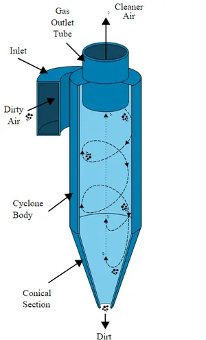
Cyclone separators work much like a centrifuge, but with a continuous feed of dirty air. In a cyclone separator, dirty flue gas is fed into a chamber. The inside of the chamber creates a spiral vortex, similar to a tornado. This spiral formation and the separation is shown in Figure . The lighter components of this gas have less inertia, so it is easier for them to be influenced by the vortex and travel up it. Contrarily, larger components of particulate matter have more inertia and ar not as easily influenced by the vortex.
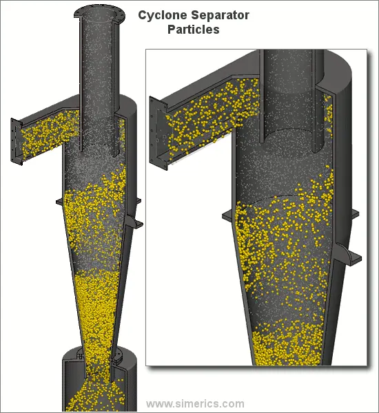
Since these larger particles have difficulty following the high-speed spiral motion of the gas and the vortex, the particles hit the inside walls of the container and
drop down into a collection hopper. These chambers are shaped like an upside-down cone to promote the collection of these particles at the bottom of the
container. The cleaned flue gas escapes out the top of the chamber.
Four empirical models used to calculate the cyclone separator efficiency :
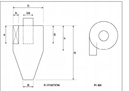
OZIA AND LEITH MODEL:
Iozia and Leith (1990) logistic model is a modified version
of Barth (1956) model which is developed based on force
balance. The model assumes that a particle carried by the
vortex endures the influence of two forces: a centrifugal force,
Z, and a flow resistance, W. Core length, zc, and core diameter ,dc are given as:
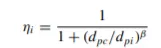
β is an expression for slope parameter derived based on the
statistical analysis of experimental data of a cyclone with D = 170
0.25 m given as:

and dpc is the 50% cut size given by Barth:
where core length zc and core diameter dc are given as
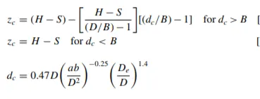
Li and Wang Model :
The Li and Wang [3] model includes particle bounce or reentrainment and turbulent diffusion at the cyclone wall. A twodimensional analytical expression of
particle distribution in the cyclone is obtained. Li and Wang model was developed based 180 on the following assumptions:
The radial particle velocity and the radial concentration profile are not constant for uncollected particles within the cyclone.
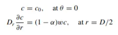
Boundary conditions with the consideration of turbu185 lent diffusion coefficient and particle bounce reentrainment on the cyclone wall are:
Koch and Licht Model:
Koch and Licht [2] collection theory recognized the inherently turbulent nature of cyclones and the distribution of gas
residence times within the cyclone. Koch and Licht described
particle motion in the entry and collection regions with the ad- 200
ditional following assumptions:
• The tangential velocity of a particle is equal to the tangential velocity of the gas flow, i.e. there is no slip in the
tangential direction between the particle and the gas.
• The tangential velocity is related to the radius of cy- 205
clone by: u Rn = constant.
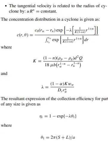
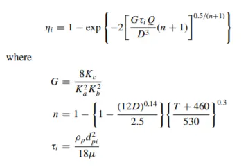
A force balance and an equation on the particles collection yields
the grade efficiency ηi:
Lapple Model:
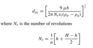
Lapple [1] model was developed based on force balance without considering the flow resistance. Lapple assumed that a par215 ticle entering the cyclone is
evenly distributed across the inlet opening. The particle that travels from inlet half width to the wall in the cyclone is collected with 50% efficiency. The semi
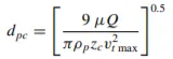
empirical relationship developed by Lapple [1] to calculate a 50% cut diameter, dpc, is:
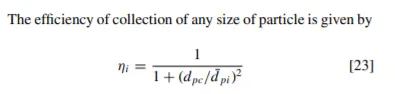
The collection efficiency of cyclones varies as a function of density, particle size andcyclone design. Cyclone efficiency will generally increase with increases in particle size and/or density; inlet duct velocity; cyclone body length; number of gas revolutions in the cyclone; ratio of cyclone body diameter to gas exit diameter; inlet dust loading; smoothness of the cyclone inner wall.Similarly, cyclone efficiency will decrease with increases in the parameters such as gas viscosity; cyclone body diameter; gas exit diameter; gas inlet duct area; gas density; leakage of air into the dust outlet.
The efficiency of a cyclone collector is related to the pressure drop across the collector.
This is an indirect measure of the energy required to move the gas through the system.
The pressure drop is a function of the inlet velocity and cyclone diameter. Form the
above discussion it is clear that small cyclones are more efficient than large cyclones.
Small cyclones, however, have a higher pressure drop and are limited with respect to
volumetric flow rates. Another option is arrange smaller cyclones in series and/or in
parallel to substantially increase efficiency at lower pressure drops. These gains are
somewhat compensated, however, by the increased cost and maintenance problems. Also
these types of arrangements tend to plug more easily. When common hoppers are used in
such arrangements, different flows through cyclones can lead to reentrainment problems.
modeling approach:
there are 5 steps in the modeling approach.
1. geometry correction(using space claim).
2. meshing. (using Ansys mesher).
3. setup problem.(using Ansys fluent).
4. solution using(Ansys fluent).
5. results.(using CFD post).
geometry preparation:
Geometry:
Fluid Volume extracted using SpaceClaim is shown below:
Mesh details
Size Function: Proximity & Curvature
Min Element Size: 10mm
No of Nodes: 113728
No of Elements: 59175
Boundary Conditions:
Inlet & outlets are as shown above.
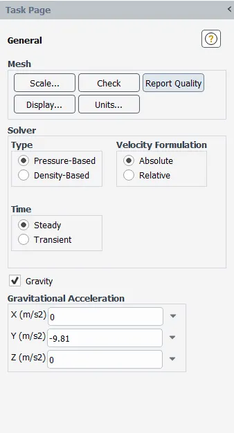
Gravity is enabled in the -ve y-direction.
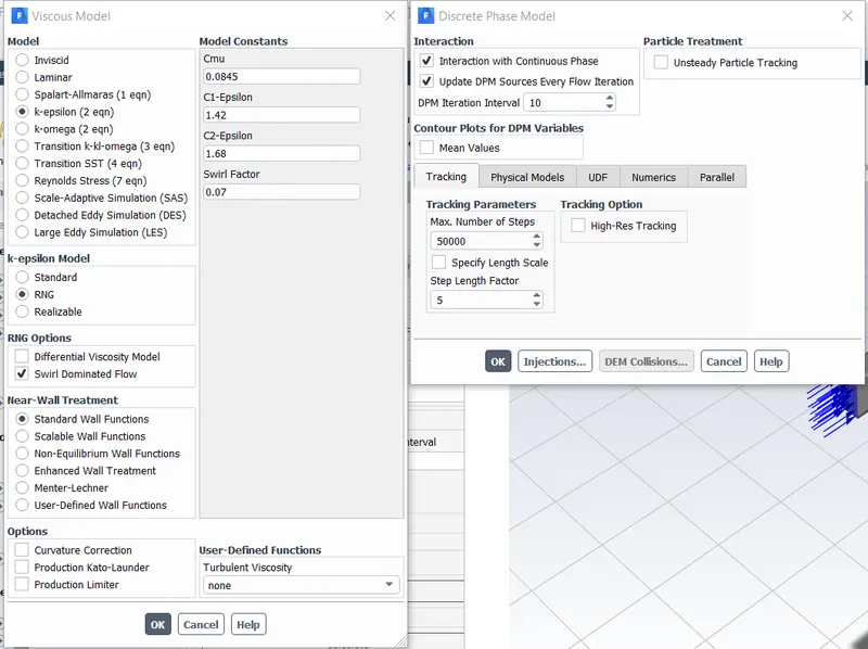
The swirl dominated RNG K-epsilon model is used here to capture the flow more accurately.
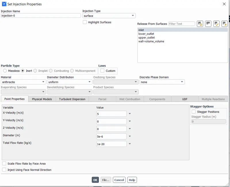
The Discrete phase modeling is used to track the flow of the particles.
No of step for particle tracking = 50000
Injection Material : Anthracite (5microns in diameter)
Velocity Inlet: 3m/s
Outlet: Pressure Outlet( Gauge Pressure= 0Pa)
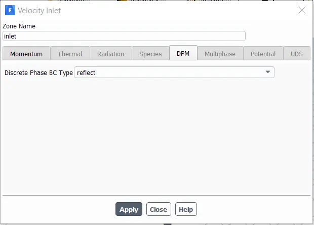
DPM Settings are varied b/w reflect,escape, trap & wall jet.
Reflect: The particle rebounds off the boundary in question with a change in its momentum as defined by the coefficient of restitution.
Escape: Particle escapes out when encountered by the boundary.
Trap: The trajectory calculation is terminated & fate of the particle is recorded as a trap.
Wall-Jet: The wall-jet type boundary condition is applicable for high-temperature walls where no significant liquid film is found & high Weber No impacts whenthe spray acts as a jet. This model is not applicable to regimes where the film is important.
solution approach and solver requirement:
results:
case(1)
in this case, we are making the velocity constant and we are visualizing the difference in results for different particle size
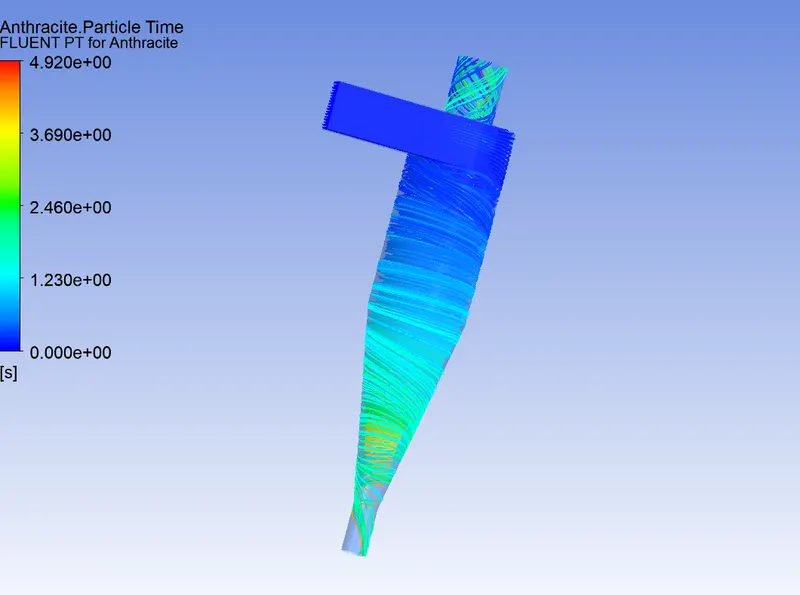
results for the particle size of 1 micron with a velocity of 3m/s
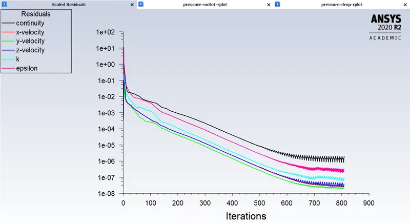
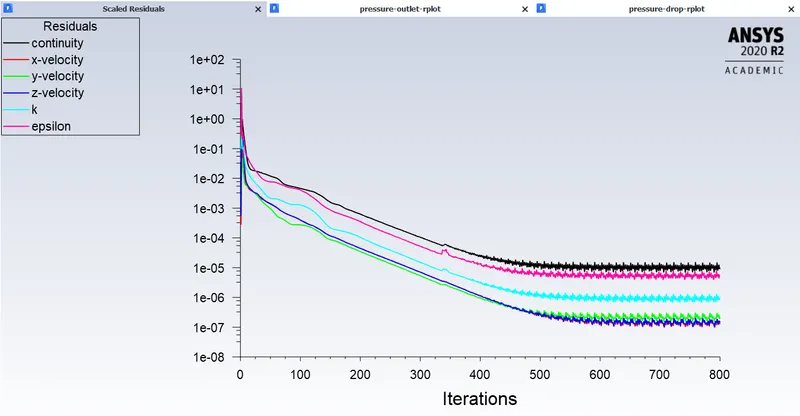
Residual Graph
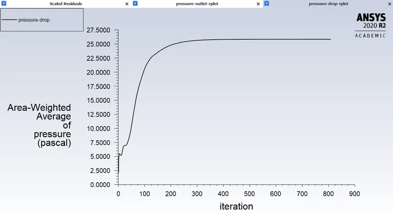
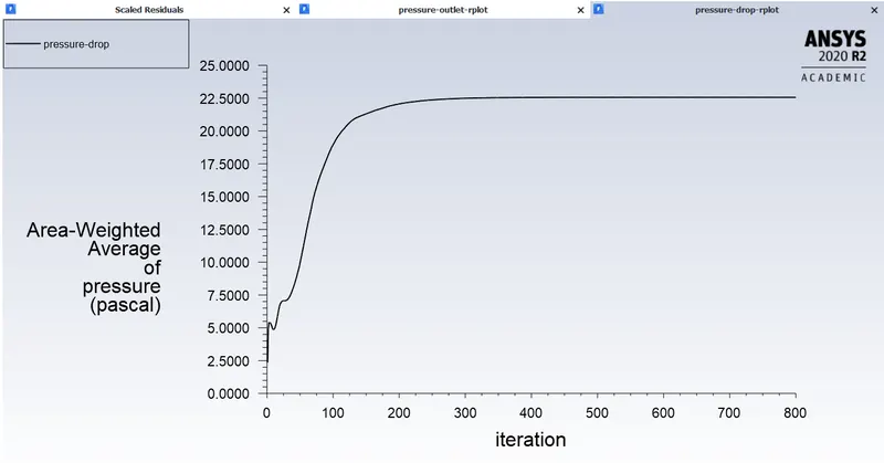
Pressure at inlet
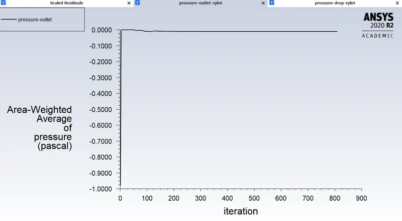
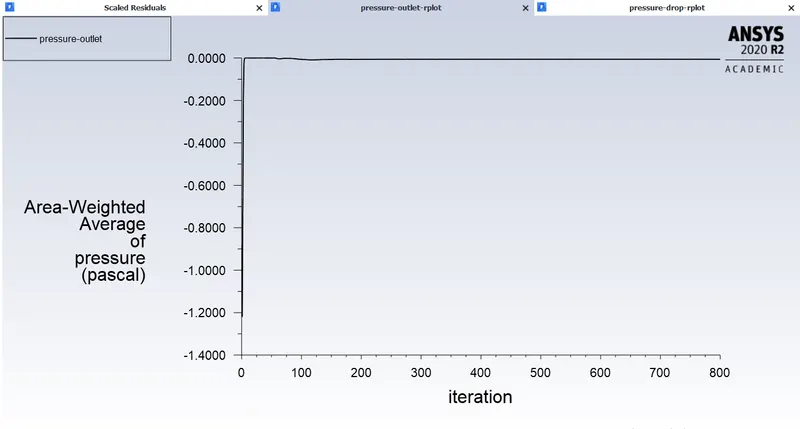
Pressure at outlet
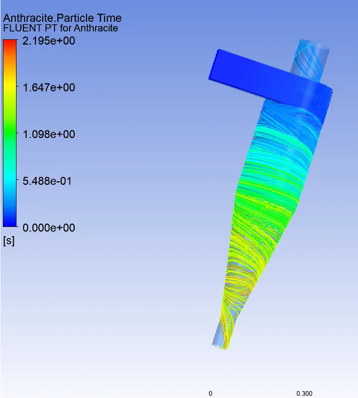
Particle tracking

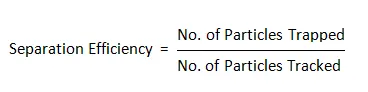
Separation Efficiency in % = (52 / 98) * 100
Separation Efficiency = 53.06 %
results for the particle size of 2 micron with a velocity of 3m/s .
residuals graph:
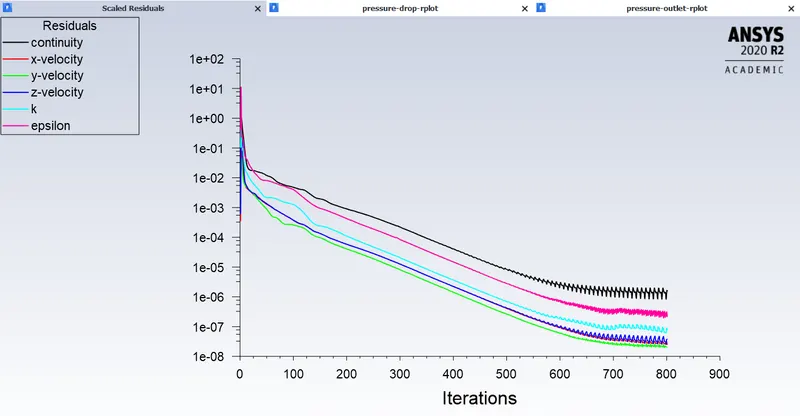
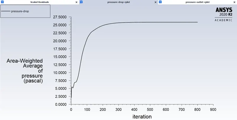
Pressure inlet
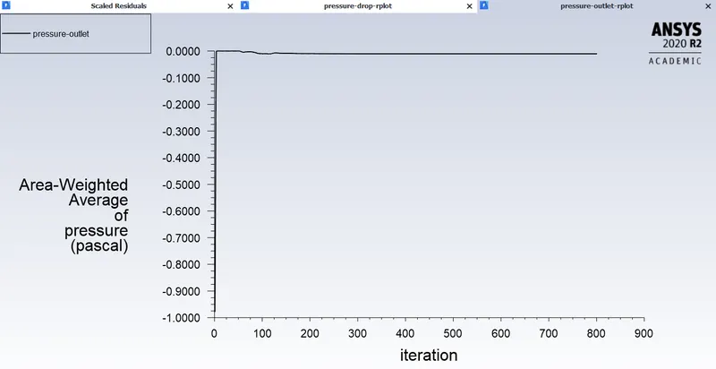
Pressure outlet
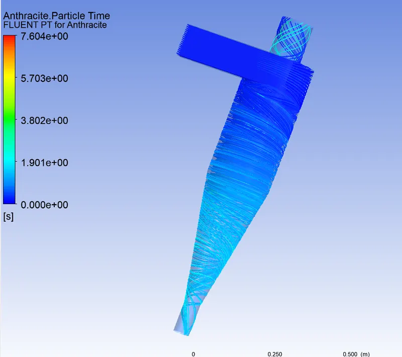
Particle Tracking

Separation Efficiency in % = (75 / 98) * 100
Separation Efficiency = 76.53 %
results for the particle size of 5 micron with a velocity of 3m/s .
residuals graph:
residual graph
Pressure at inlet
Pressure at outlet
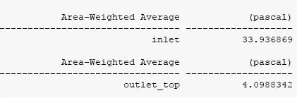
Total pressure
Now,
Pressure drop = Total inlet pressure - Total Outlet Pressure
= 33.93 – 4.099
Pressure drop =29.83 Pa
Particle Tracking:

Separation Efficiency in % = (98 / 98) * 100
Separation Efficiency = 100 %
case(2)
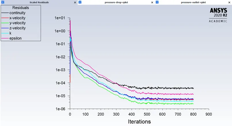
results for the varying velocity and kepping the particle size constant i.e 5 micron
inlet velocity of the particle and the discrete phase is same i.e 1m/s
residuals graph:
pressure at inlet:
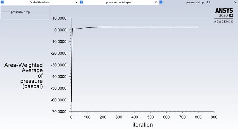
pressure at outlet:
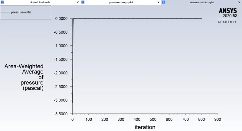
Total pressure
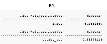
Pressure drop = Total inlet pressure - Total Outlet Pressure
= 3.15 – 0.36
Pressure drop =2.79 Pa
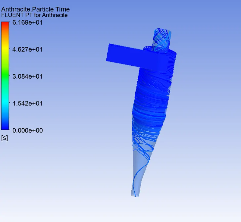
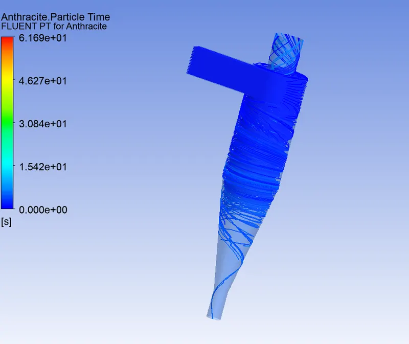
Particle Tracking:

Separation Efficiency in % = (7 / 98) * 100
Separation Efficiency = 7.14 %
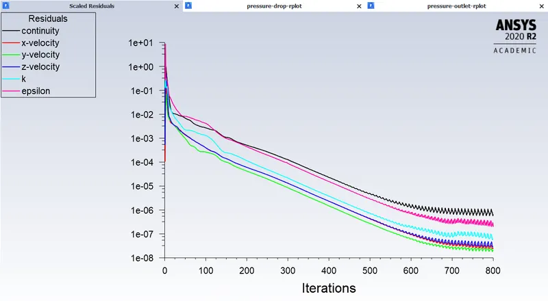
inlet velocity of the particle and the discrete phase is same i.e 3m/s
residuals graph:
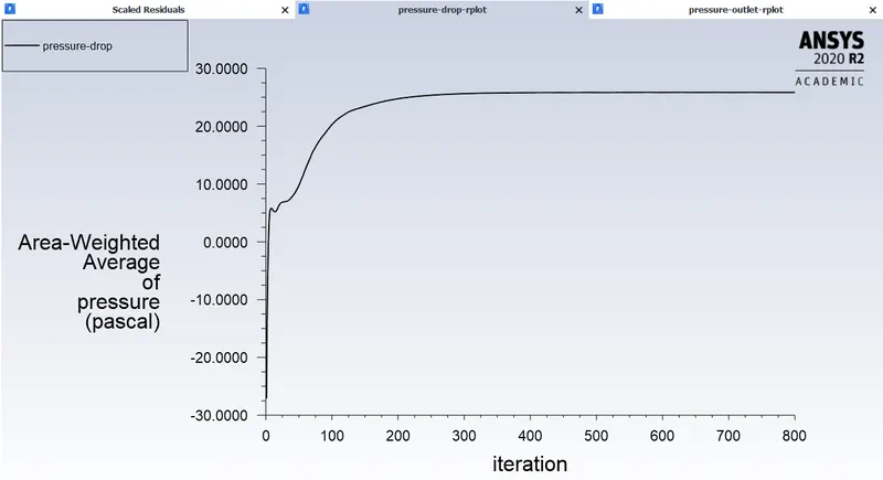
pressure at inlet:
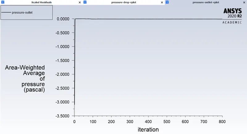
pressure at outlet:
Total Pressure:
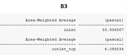
Pressure drop = Total inlet pressure - Total Outlet Pressure
= 33.93 – 4.09
Pressure drop =29.83 Pa
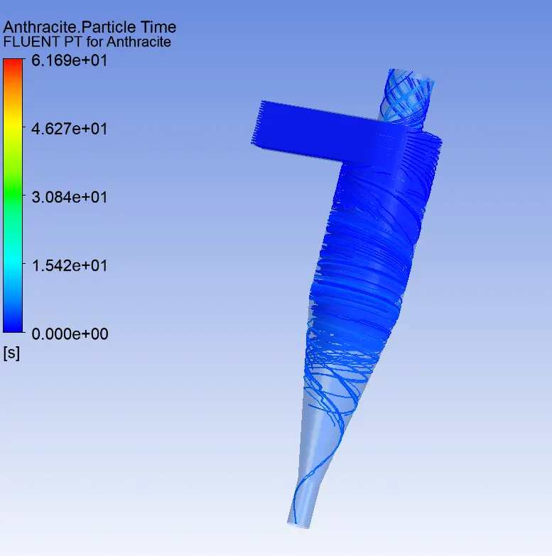
Particle Tracking:

Separation Efficiency in % = (98 / 98) * 100
Separation Efficiency = 100 %
et velocity of the particle and the discrete phase is same i.e 5m/s
Residual graph
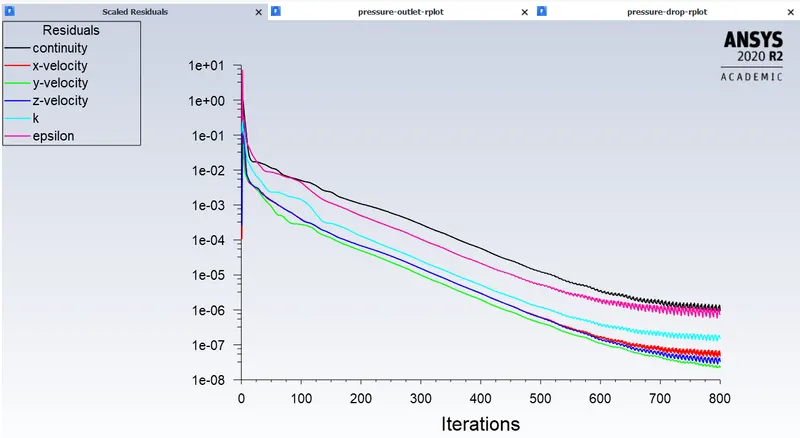
Pressure at inlet
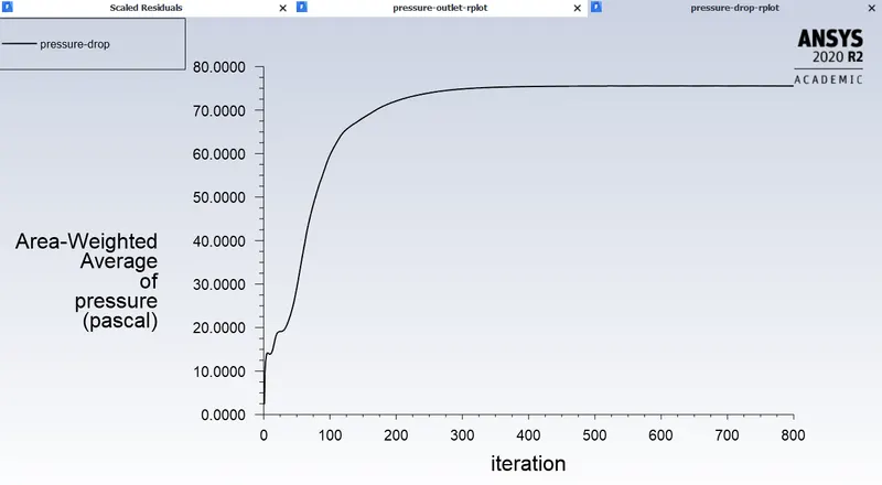
Pressure at outlet
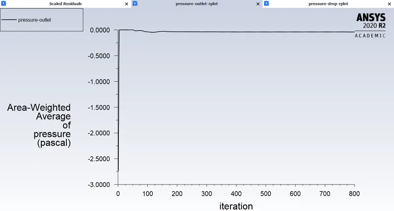
Total Pressure
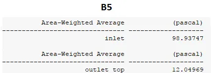
ressure drop = Total inlet pressure - Total Outlet Pressure
= 98.93 – 12.04
Pressure drop =86.89 Pa
Particle Tracking:

Separation Efficiency in % = (98 / 98) * 100
Separation Efficiency = 100 %