Week - 8 Mass Scaling

Mass Scaling through time-step control

Aim: To study the effect of time-step size on the computation time and control mass error or percentage mass addition to the model to limit it to 8%. The stability of the simulation is to be ensured i.e. the model should behave the same with and without mass-scaling. Finally, the simulation is run with an implicit solver to note the difference in computation time.

Theory: The stability time-step size in an explicit dynamic analysis is given by the Courant-Fredrick-Levit equation:

`delta`t < L.`square root`(`rho`(1-2`nu`)/(2`mu`(1-`nu`))..........................(i)

This is the time taken by a sound wave to travel through the length (L) of an element having material density `rho`, Poisson's ratio `nu`, and viscosity `mu`. Equation (i) basically calculates the time it takes for a stress wave, traveling at the speed of sound (determined by its material properties) to cross an element of length L. In LS-Dyna, the minimum time step is either allowed to be computed automatically or fed by the user. In either case, if the time step in the simulation falls below this minimum threshold, the time step is increased by adding mass to the element - which increases its density `rho` and consequently, by equation (i), its time step. This mass addition needs to be kept in check -below a certain percentage of the total mass of the system - since it is artificial mass being added and will distort the energy balance in the system such that the energy ratio at the end of the simulation is more than 1. The results obtained will not be reliable and relatable to the actual physical problem.

Geometry and spatial discretization: The geometrical model consists of a plate 33.02m in length and width and 3.124m thick with a 2.54m slit running through the center and diverging into 7.3m at the edge of the plate. The upper and lower halves, each have a 6.35m hole with a 5.805m cylindrical pin running through them. The lower pin is intended to remain fixed (and in contact with the hole) and the upper pin is intended to displace upwards thereby trying to induce a tensile tear through the centerline.

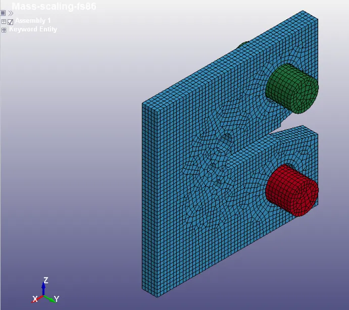
Fig 1: Geometrical Model with Mesh

The model (plate and pins) is meshed with 13505 solid hex dominant elements with an ELFORM of 1 - constant stress solid element. Additionally, a global hourglass control with IHQ = 6 - Belytschko-Bindeman assumed co-rotational stiffness form for 2D and 3D solid elements - is used.

Constitutive Material Model: The plate is provided with a piecewise-plastic material model with the following properties:

Sl No	Material Property	Magnitude	Unit
1	Density	7830	kg/m3
2	Young's Modulus	2.00e+11	Pa
3	Poisson's Ratio	0.27	-
4	Yield Stress	1.113e+09	Pa

Table1: Piecewise-Plasticity Material Model Properties

The plasticity region is defined using the stress-strain curve shown below:

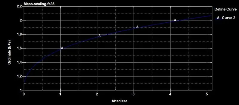
Fig 2: Stress-Strain curve of the plastic region of piecewise plastic material model

The pins are provided with a MAT_Rigid material card with the following properties:

Sl No	Material Property	Magnitude	Unit
1	Density	8000	kg/m3
2	Young's Modulus	2.00E+11	Pa
3	Poisson's Ratio	0.3	-

Additionally, using the CMO, CON1, and CON2 options the pins are constrained to allow translation in the global Z-direction only.

Contact Definition: For the explicit runs, Automatic_Surface_Surface contacts are defined between the pins' upper and lower surfaces and the corresponding surface of the holes - through the creation of segments. A static coefficient of friction of 0.05 was defined for the contacts.

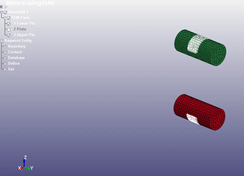
Fig 3: Contact elements on the pins

For the implicit run, this contact is replaced with Automatic_Surface_Surface_Mortar contact with similar definitions as mentioned above.

Boundary Conditions: The lower pin is constrained along all the axes in translation only. The upper pin is constrained along the X and Y directions only. These constraints are defined using Boundary_SPC.

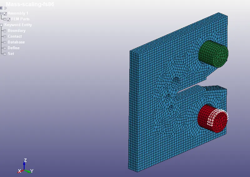
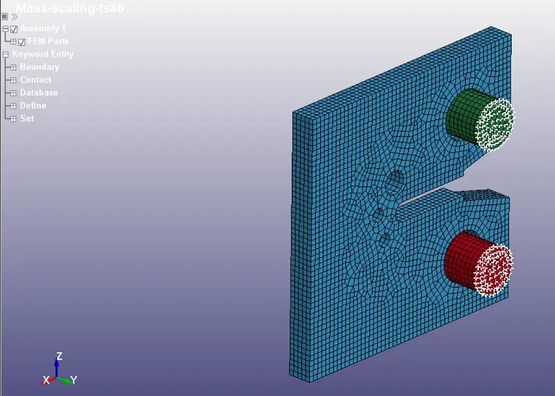
Fig 4: Lower pin SPC - all translational DOF locked Fig 5: Upper pin SPC - X and Y translational DOF locked

The upper pin is also provided a velocity of 1.27e-05m/s along the positive Z-direction through Boundary_Prescribed_Motion.

For the implicit run, 'negative eigenvalue' errors were encountered during the run indicating unconstrained rigid body motion. To rectify this, the SPCs were deleted and an additional MAT_Rigid material card was added with the same properties as the first one but with constraints along all translational and rotational degrees of freedom. This card was assigned to the lower pin.

Simulation Settings: For the explicit run, the time step is altered from 1e-05s to 1.1e-04s. The corresponding computation time and mass errors are noted. The termination time is set to 600s and all simulations are run with 4SMP threads.

For the implicit run, the implicit solver is triggered using Implicit_General. Time-step and iteration range is set using Implicit_Auto. A constant time-step of 1s was used to have the same number outputs written for the animation file. A non-linear BFGS update with an optional arc-length update scheme is used for the solver. The displacement convergence tolerance is set to 0.001 with consideration for the total displacement in the model over the entire time duration. For better convergence, IACC is set to 1 in Implicit_Accuracy. The parameters of the Implicit_Solver card are left to their default values.

Results and Discussion: The explicit simulation computation times and %mass addition are noted for each time-step size and the results are plotted. The resulting plots are as shown in Fig 7 and 8.

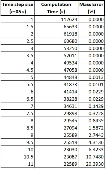
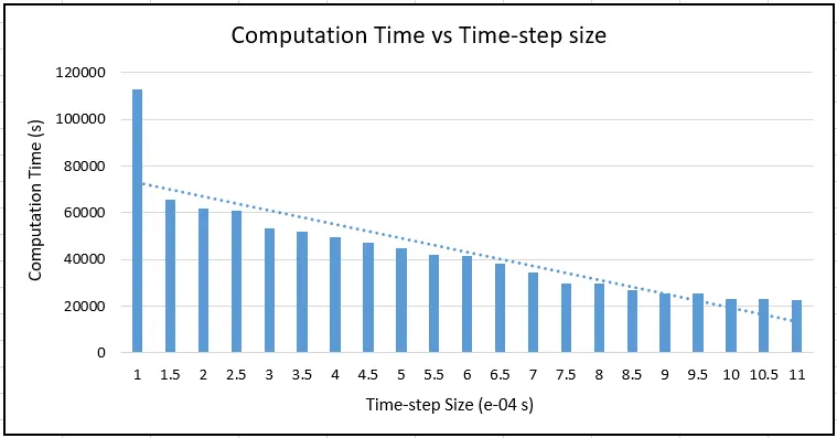
Fig 6: Results Data Fig 7: Computation time histogram

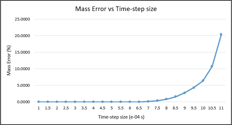
Fig 8: Line Plot for % Mass addition

From Fig 7, it can be observed that the computation times decrease with increasing time-step size, as shown by the dotted trendline. It should be pointed out here that the computation times noted here are from the initial estimates that show up on the solver screen when the simulation starts. These estimates are usually not accurate and the actual simulation times are a lot less than initially projected.

Mass Error or % Mass Addition on the other hand stays zero up to 4.5e-05s and then starts increasing. The increase is not proportional and the error jumps from 6.4233% to 10.748% when the time step increases from 1e-04s to 1.05e-04s. The simulation results for the model with mass-scaling (within 8%) and the model without mass-scaling are almost in agreement with each other (as can be seen from the animations below).

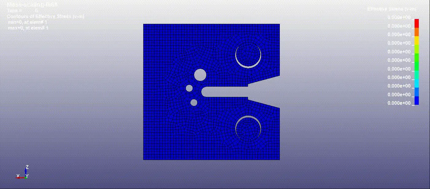
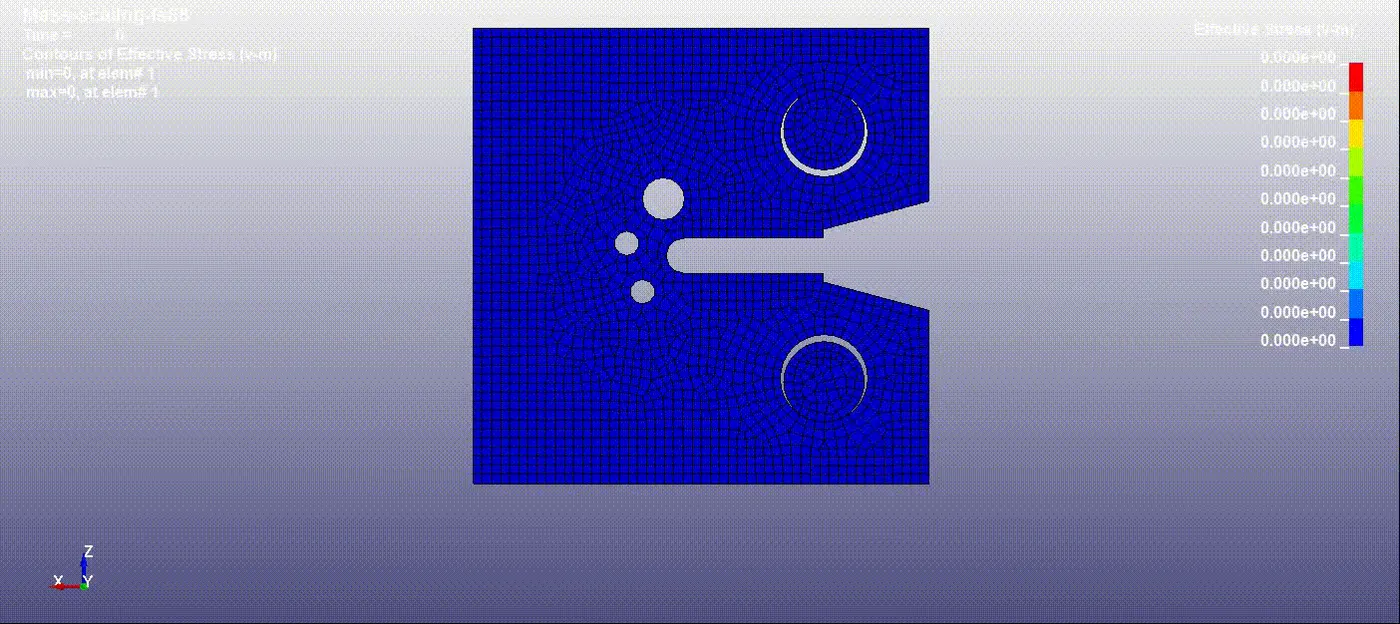
Fig 9: Von-Mises stress fringe plot without mass-scaling Fig 10: Von-Mises stress fringe plot with mass-scaling

The implicit run was solved within 3520s or 58mins and 40 secs in contrast to the explicit runs where the lowest estimated time was 22589s or 6hrs and 20mins.

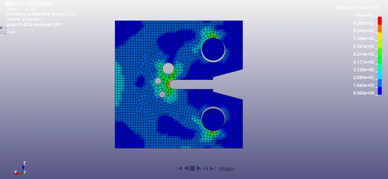
Fig 11: Von-Mises stress fringe plot for implicit run

Conclusion: For the given non-linear static problem, the implicit approach solves the problem much faster than the explicit mode. This is because in the explicit analysis, the stability of the run depends on the time-step respecting the CFL condition which in turn is dictated by the smallest element length in the model. This value is very small - of the order of e-05 without mass-scaling. This extremely small time-step size leads to very high computation time. In case of the implicit run, the time step size is not stability dependent and can therefore be larger. The only limit to this would be convergence issues which would demand a lower time-step. In this particular case, the load is static i.e. the acceleration of the upper pin is almost constant throughout the run, and the existing non-linearities - contact and material- are also not extreme in nature. Therefore, the problem does not demand a very small time step and is solved using a much larger time-step leading to a shorter total computation time.

It can also be observed from Fig 11 that the stress results of the implicit run differs vastly from the explicit run. This is due to the implicit code trying to reduce the residual norm at each iteration and converge the results.