MASS SCALING IN LS-DYNA

Objective:

One of the most important techniques in CAE industry to reduce the run time of an explicit FE analysis is 'Mass Scaling'.

The main objective of this report is to make use of mass scaling technique to effectively reduce the simulation run time and to ensure the stability of mass scaling.

With a mass scaling percentage limit of 8 and by optimizing the mass scaling parameters 'Timestep' and 'TSSFAC' (Timestep scaling factor), many trials have been undergone to achieve reduction in simulation run time.

Also, to perform an implicit analysis simulation for the same model and to compare the running time between explicit and implicit methods.

Mass Scaling:

Mass scaling refers to a technique whereby a non-physical mass is added to a structure in order to achieve a larger explicit timestep.

The run time of an FE simulation is mainly a function of model size and size of the solution step.

As the size of the model is not in our control, we have to play with varying timestep. Thus bigger the timestep, faster the simulation is.

But,fixing the range of bigger timestep depends on the sensitivity of the model and accuracy required.

As per Courant-Friedrichs condition for explicit analysis is

,where `Deltat` is the timestep, `e_min` is the size of the smallest mesh element and `c` is the speed of stress wave.

The scaling factor is used for providing numerical stability to the solution.

Also,

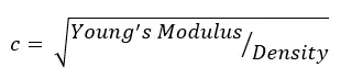
If we increase the density of small element, we get an increased timestep.Henceforth, reducing the solution run time.

Mass scaling procedure in LS-DYNA:

LS-DYNA allows two different types of mass-scaling using the DT2MS parameter from *CONTROL_TIMESTEP with the default set to no mass-scaling.

When DT2MS is less than zero, LS-DYNA adds mass of each element whose timestep is below abs(DT2MS) such that the element's updated DT is equal to abs(DT2MS).

When DT2MS is greater than zero, LS-DYNA adds mass to elements whose DT is below abs(DT2MS) and "removes" mass from elements whose DT is greater than zero.

DT2MS>0 is seldom used while DTM2<0 is frequently used for overcoming the smallest computed timestep.

Care must be taken when using DT2MS<0 to ensure that the added mass does not have an adverse effect on the simulation accuracy

In this projectwork, the simulation is carried out initially without mass scaling to find the default computational time, then by varying the mass scaling parameters to reduce the simulation run time.

Without mass scaling:

Firstly, the simulation is set to run in LS-DYNA manager without any mass scaling parameters to know the default computational time.

It is found that the run time for simulation without mass scaling is `329407 sec` which is `91.5 hrs`.

This is such a huge time period for the simulation to run.

Hence, certain mass scaling techniques have been imposed to reduce the run time of simulation.

Mass scaling with variable timestep and constant TSSFAC=0.9

Using the card *CONTROL_TIMESTEP, we define the value for timestep for each trial and a constant TSSFAC value of 0.9.

1.Timestep = 7.5E-05

It is found that, using these timestep paramaters, the mass scaling is about `0.3728%` and the run time of the simulation is `88888sec` which is `24.69 hrs`.

It can be seen that the run time value tends to decrease when comparing with previous default simulation.

2.Timestep = 5.5E-05

Here, the mass scaling is about `0.01%` and the simulation run time is `127823sec`which is `35.5hrs`.

Likewise, many trials have been undergone to reach a mass scaling limit of `8%` that gives a reduced run time of the simulation.

The following tabular data gives represents the mass scaling percentage trials with respect to run time of simulation.

Explicit analysis with TSSFAC = 0.9
S.No	Timestep	Mass scaled %	Run time (sec)	Run time (Hours)
1	-0.000075	0.3728	88888	24.69111111
2	-0.000055	0.010034	127823	35.50638889
3	-0.000035	0	136221	37.83916667
4	-0.0001	6.4233	70302	19.52833333
5	-0.00010285	7.9747	58926	16.36833333
6	-0.0001025	7.766	73909	20.53027778
7	-0.0001005	6.6718	73571	20.43638889
8	-0.000103	8.066	78846	21.90166667
9	-0.000102	7.4771	64766	17.99055556
10	-0.000101	6.9297	84608	23.50222222

From the above table, it is found that with a timestep value of `-1.0285 E-04`, we get a mass scaling limit of `8%` with low computational time of `16.368 hrs`.

Mass scaling with variable timestep and constant TSSFAC=0.8

The above procedure is repeated for same variabe timestep values and TSSFAC value of 0.8.

1.Timestep = 7.5E-05

It is found that, using these timestep paramaters, the mass scaling is about `0.3728%` and the run time of the simulation is `128181sec` which is `35.6 hrs`.

2.Timestep = 5.5E-05

It is found that, using these timestep paramaters, the mass scaling is about `0.01%` and the run time of the simulation is `142561sec` which is `39.6 hrs`.

Also, it is noted that,with the variation of TSSFAC parameter, there is no change in the mass addition.This means that irrespective of TSSFAC values,the run time is influenced by variation timestep.

Likewise, many trials have been undergone to reach a mass scaling limit of `8%` that gives a reduced run time of the simulation.

The following tabular data gives represents the mass scaling percentage trials with respect to run time of simulation.

Explicit analysis with TSSFAC = 0.8
S.No	Timestep	Mass scaled %	Run time (sec)	Run time (Hours)
1	-0.000075	0.3728	128181	35.60583333
2	-0.000055	0.010034	142561	39.60027778
3	-0.000035	0	140710	39.08611111
4	-0.0001	6.4233	74999	20.83305556
5	-0.00010285	7.9747	62345	17.31805556
6	-0.0001025	7.766	83148	23.09666667
7	-0.0001005	6.6718	95658	26.57166667
8	-0.000103	8.066	72153	20.0425
9	-0.000102	7.4771	73529	20.42472222
10	-0.000101	6.9297	73582	20.43944444

From the above table, it is found that with a timestep value of `-1.0285 E-04`, we get a mass scaling limit of `8%` with low computational time of `17.31 hrs`.

It is to be noted that while changing the scaling factor from 0.9 to 0.8, the run time seems to increase (i.e.run time with TSSFAC=0.8 is greater than run time with TSSFAC=0.9).

Thus, decreasing the TSSFAC value, tend to increase the run time of the simulation which is not appreciated.

Hence, with `Time step=` `-1.0285E-04` and `TSSFAC=` `0.9` gives the lowest simulation run time.

Comparison:

A histogram chart is prepared that reveals the run time of the simulation with respect to timestep for mass scaling trials.

It is seen that with a timestep of -1.0285E-04 and TSSFAC of 0.9, the simulation has the least run time.

Implicit analysis:

The same simulation is set to run with implicit analysis in LS-DYNA.

With all other cards(*MATERIAL, *SECTION,*CONTACT, *CURVE) as default except *CONTROL cards, there made some changes accordingly to perform implicit analysis.

Using *CONTROL_IMPLICIT_GENERAL card, implicit analysis is activated with IMFLAG=1 and with initial timestep as 1 (i.e.DT0=1).

Using *CONTROL_IMPLICIT_AUTO card with IAUTO=1, the timestep size is automatically adjusted.

Using *CONTROL_IMPLICIT_SOLUTION card, the implicit analysis is used to choose between linear and non-linear analysis.

Using *CONTROL_IMPLICIT_SOLVER card, where the stiffness matrix invesion takes place, LSOLVR=4 is used to solve the simulation with single precision which consequently saves run time rather than going for double precision solver.

The simulation is solved and the computational time is noted.

It is found that the implicit method took `1839sec` which is `30min` to solve.

The reason for much shorter run time is that because of initial timestep of 1 and is used with constant timestep formulation since our termination time is very large.

Again, while accounting for accuracy, the timestep for implicit analysis should be well considered.

Conclusion:

Mass-scaling is a term that is used for the process of scaling the element's mass in explicit simulations to adjust its timestep.

The primary motivation is to increase the global compute timestep which is limited by the Courant's stability criteria.

Implicit and Explicit analysis differ in the approach to time increments.

In Implicit analysis each time increment has to converge, but we can set pretty long time increments. Explicit on the other hand doesn’t have to converge each increment, but for the solution to be accurate time increments must be super small.

Both implicit and explicit analysis does more or less the same thing. They divide the analysis time into small increments, and then analyze what is going on in our model one increment of time after another.

The speed of computing is exactly the difference between implicit and explicit.

Though the running time for implicit analysis is shorter than explicit analysis method, the debate on what type of solver is better depends upon the type of problem and accuracy we need.