Week - 8 Mass Scaling
Assignment 8
The objective of this assignemnt is to run a simulation in its original state (without changing paramenters that affect tha mass-scaling). After running the simulation, the parameters should be adjusted to minimize the computation time. In the end, there will be a comparison between all the results obtained for the simulation.
1. Setting up and running the initial simulation
First, to achieve a faster and more efficient result acquisition, the total time of the simulation was changed from 600 s to 10 s. This reduction still allowed one to understand the behaviour of the deformed component as well as ensuring that more simulations were carried, so that a more precise parameter optimization was obtained.
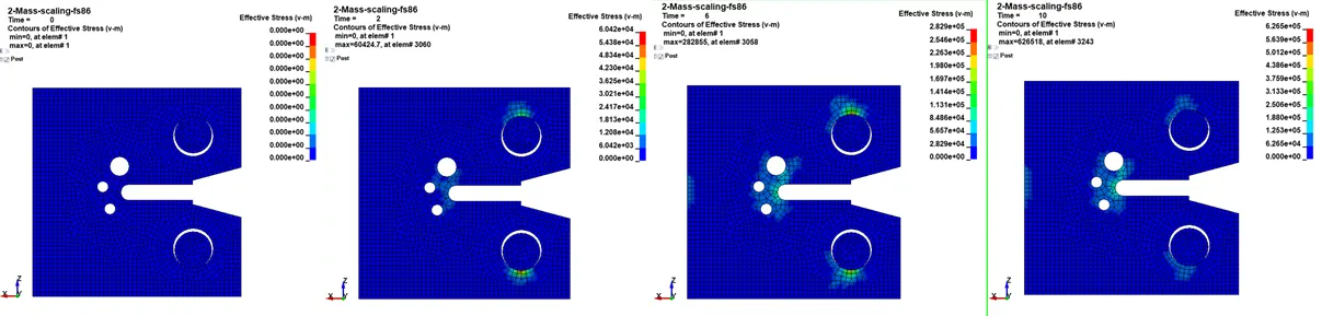
The results of the first simulation correspond to the expectations. The stress concentration appear in the expected areas (contact with the rigid cylinders and groove).
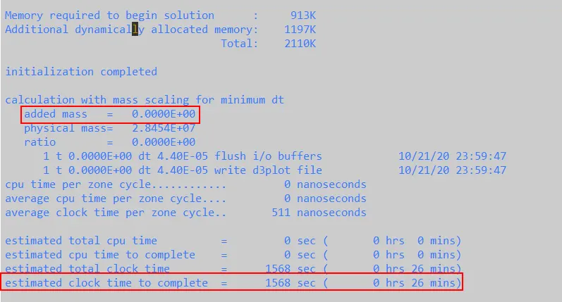
By checking the .out file, it was confirmed that no mass was added to the model. And that the computation time was 1568 s, as shown below.
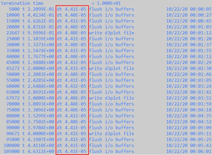
The negative value for DT2MS means that only time steps that are smaller than the absolute value of DT2MSxTSSFAC are increased by mass-scaling to match the value of DT2MSxTSSFAC.
It was conculded that the time step used by the program was always between 4.40e-5 and 4.41e-5 m, which is greater than the value set for DT2MS (|-3.5e-5| m).
It makes sense that no mass was added to the model in this simulation because it was not needed to correct the time step to a greater value.
Using a positive value for DT2MS will force the values of all time steps to the absolute value of DT2MSxTSSFAC, even if that means decreasing the time step. That would, eventually, contibute towards an increase of the total simulation time, which is not of our interest. For this reason, positive values of DT2MS will not be used.
2. Adjusting DT2MS
From the first simulation, it can be seen that the value of DT2MS needs to be increased. I will run the first few simulations where I will only change the value of DT2MS.
On the other hand, this is an explicit analysis, which is a conditionally stable problem. The condition that we need to impose for the time step value is the following:
`\Deltat > \frac{d_{nodes}^{min}}{c}`
Where `d_{nodes}^{min}` is the minimum distance between two nodes in the model and c is the velocity of sound in the material.
c is given by:
`c = \sqrt{\frac{E}{\rho(1-\nu^2)}} = \sqrt{\frac{E}{\rho(1-\nu^2)}} = \sqrt{\frac{200\times10^{11}}{7830(1-\0.272^2)}} = 5252 m/s `
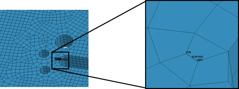
`d_{nodes}^{min}` corresponds to 0.2614 m as shown below.
So, the maximum time step allowed for an explicit analysis is:
`\Delta t^{max}= \frac{d_{nodes}^{min}}{c}=\frac{0.2614}{5252}=4.997\times10^{-5} s`
Between 4.41e-5 and 4.997e-5 there is not to much room for improvement regarding the time step. Nevertheless, the program advised that the time step should be smaller than 1.263e-4, suggesting that a different distance between nodes was used to calculate the maximum time step.
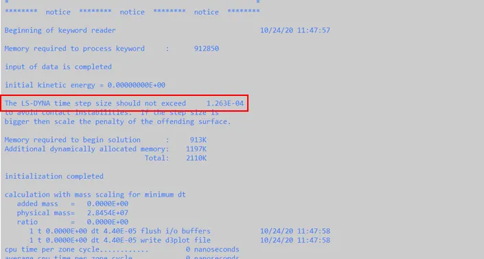
Having this in mind, I will run 4 simulations with DT2MS equal to 5e-5, 8e-5, 1e-4 and 1.2e-4 s.
The results from the simulation in terms of computation time and percentage of added mass.
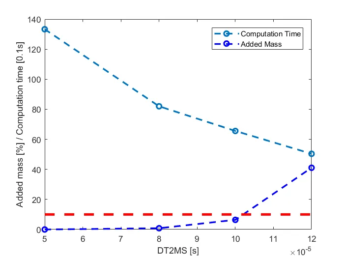
It can be concluded that the value of DT2MS that minimizes the computation time while ensuring that the maximum percentage of addded mass is not exceeded is 1e-4 s (admitting TSSFAC = 0.9).
2. Adjusting TSSFAC
6 simulations were run with the time step scale factor (TSSFAC) equal to 0.5, 0.6, 0.7, 0.8, 0.9 and 1. The results are the following
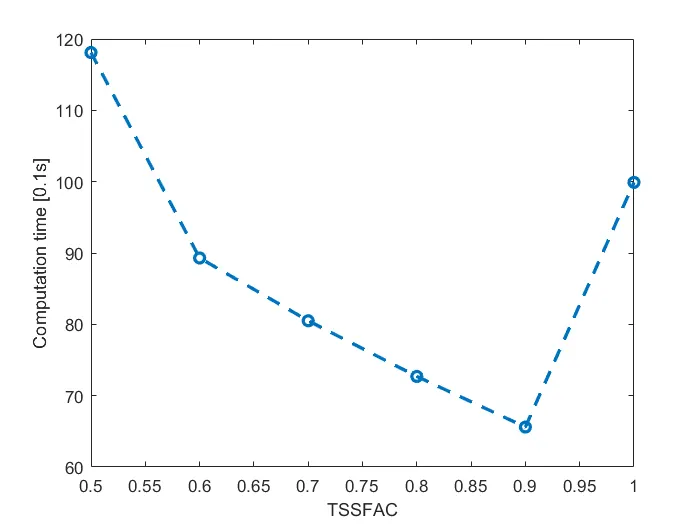
It was concluded that the most suitable value for TSSFAC was 0.9. The added mass does not depend on the value of TSSFAC, so it was not taken into consideration for this simulation.
3. Implicit simulation
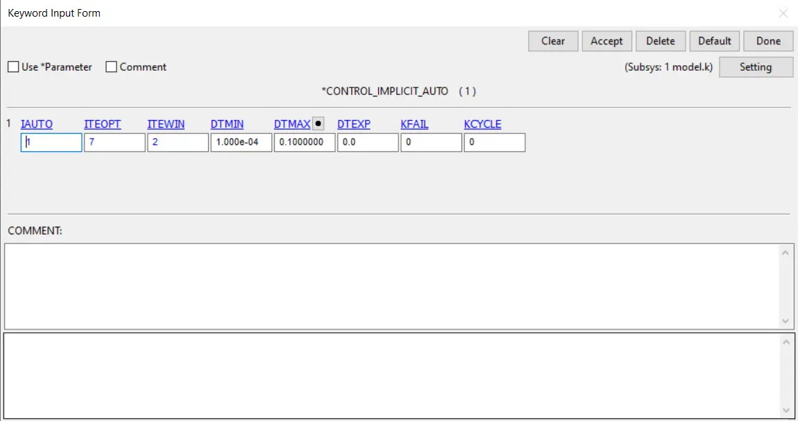
The next few images explain the implicit simulation keywords that were activated to perform this analysis
3.1. CONTROL_IMPLICIT_AUTO
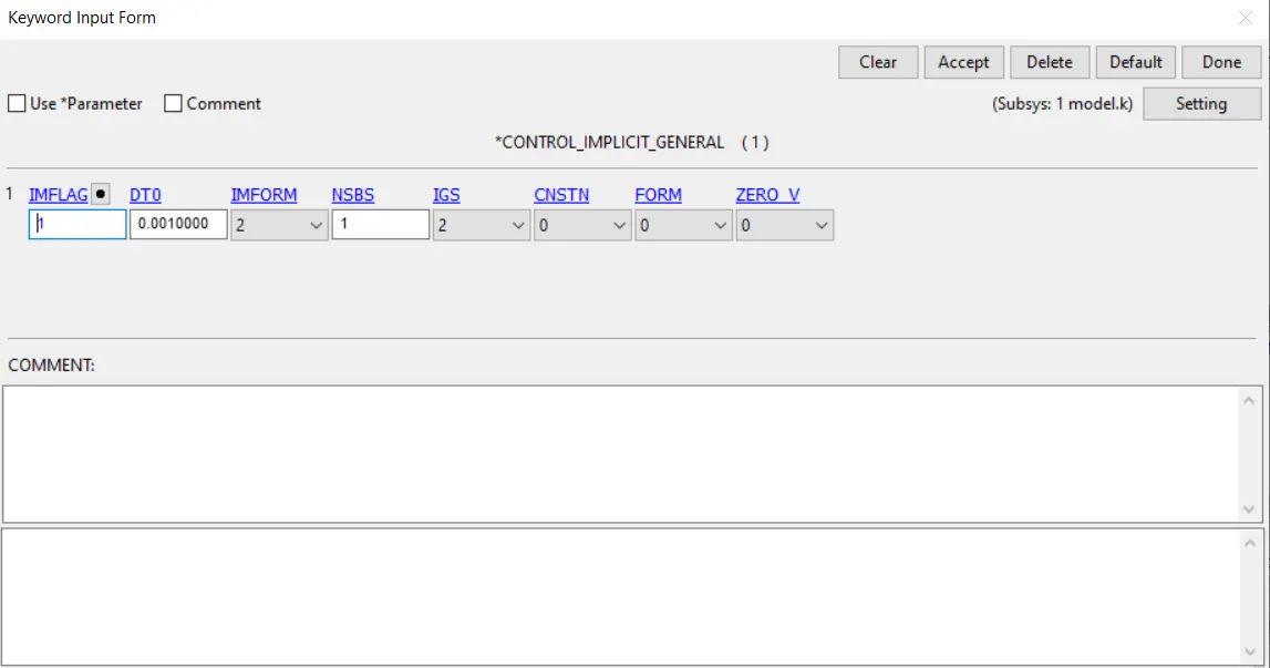
3.2. CONTROL_IMPLICIT_GENERAL
This keyword was activated to define the implicit analysis solver.
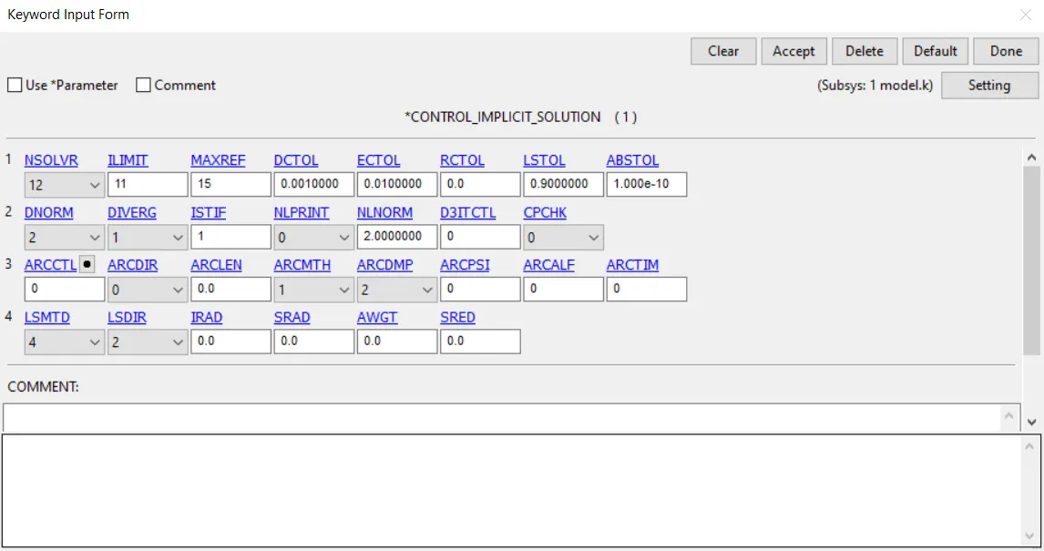
3.2. CONTROL_IMPLICIT_SOLUTION
Establishes the limit of Newton_Raphson iterations required to match tolerances of convergence for displacement.
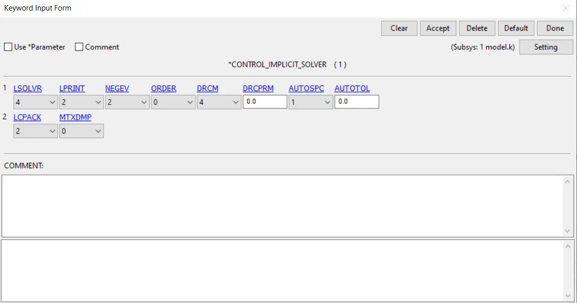
3.3. CONTROL_IMPLICIT_SOLVER
This keyword was activated to define the linear equation solver method.
4. Result comparison
In order to avoid errors in the implicit simulation, the memory option was set to 21M.
The simulation with the implicit solver took 182 seconds to run. And, by checking the .out file, the time step at which the equations were being solve corresponded to the maximum time step allowed, meaning that a larger time step could have been used and would, logically, lead to a smaller computation time.
This comparison between both techniques (explicit with mass scaling vs. implicit) comes to the conclusion that the implicit simulation has a lower computation time, that would have been even lower if the maximum time step was increased and if the non-adjustment region defined by ITEOPT and ITEWIN was optimized.