Week - 8 Mass Scaling

Mass Scaling,

Objectives,

           The purpose of this project, mass calling is reduced the simulation time. The hard limit on mass scaling is 8% and stability should be completely intact. Mass is added using DT2MS and TSSFAC (Time scale parameter should be optimized. Mass scaling objective is reached, a histogram should be plotted to compare the runtime with mass scaling trials.

Procedure,

Mass scaling, 

            Nonphysical mass to increase the timestep ina dynamic analysis, Sometimes the effects is insignificant and in those cases adding nonphysical mass is justifiable. In the explicit method, the time step usually is very small to maintain numerical stability. However, a small step size prevents this method from being useful for routine analysis work. To reduce the CPU cost and improve the performance, mass scaling is often used to increase the time step size in each cycle.

            Mass scaling invoked with DT2MS in *CONTROL_TIMESTEP. when DT2MS is the input as a negative value, mass is added only to those elements whose timestep would otherwise be less than DT2MS. The input as a positive value, mass is added or taken away from the element so that the timestep of every element is the same. My opinion is there is no advantage to using this method over the negative DT2MS method and I find it harder to rationalize.

         

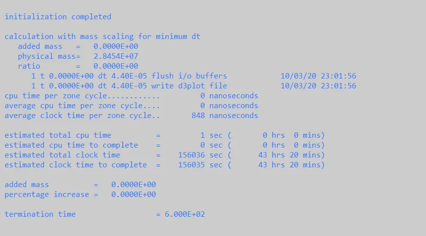
Trial 1, 

            The model have the TSSFAC and DT2MS Vaues as 0.9 and -3.5e-5 respectively. we can see estimate the simulation time in 43hr 20mins (155520sec).  

            

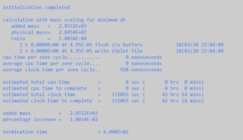
Trial 2, 

            The model have the TSSFAC and DT2MS Vaues as 0.9 and -5.5e-5 respectively. we can see estimate the simulation time in 42hr 14mins (151704sec).

             

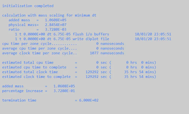
Trial 3, 

            The model have the TSSFAC and DT2MS Vaues as 0.9 and -7.5e-5 respectively. we can see estimate the simulation time in 35hr 54mins (127944sec).

              

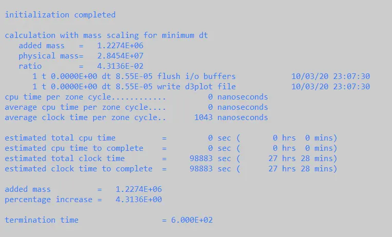
Trial 4, 

            The model have the TSSFAC and DT2MS Vaues as 0.9 and -9.5e-5 respectively. we can see estimate the simulation time in 27hr 28mins (98208sec).

                          

Trial 5, 

            The model have the TSSFAC and DT2MS Vaues as 0.9 and -1.05e-4 respectively. we can see estimate the simulation time in 24hr 12mins (84832sec).

             

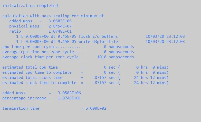
Trial 6, 

            The model have the TSSFAC and DT2MS Vaues as 0.9 and -1.02e-4 respectively. we can see estimate the simulation time in 25hr 25mins (90900sec).

             

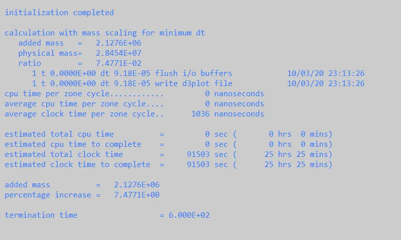
Trial 7, 

            The model have the TSSFAC and DT2MS Vaues as 0.9 and -1.021 respectively. we can see estimate the simulation time in 18hr 57mins (66852sec).

             

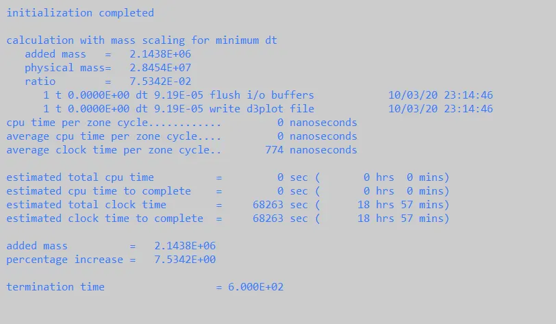
Trial 8, 

            The model have the TSSFAC and DT2MS Vaues as 0.9 and -1.022 respectively. we can see estimate the simulation time in 26hr 11mins (93996sec).

              

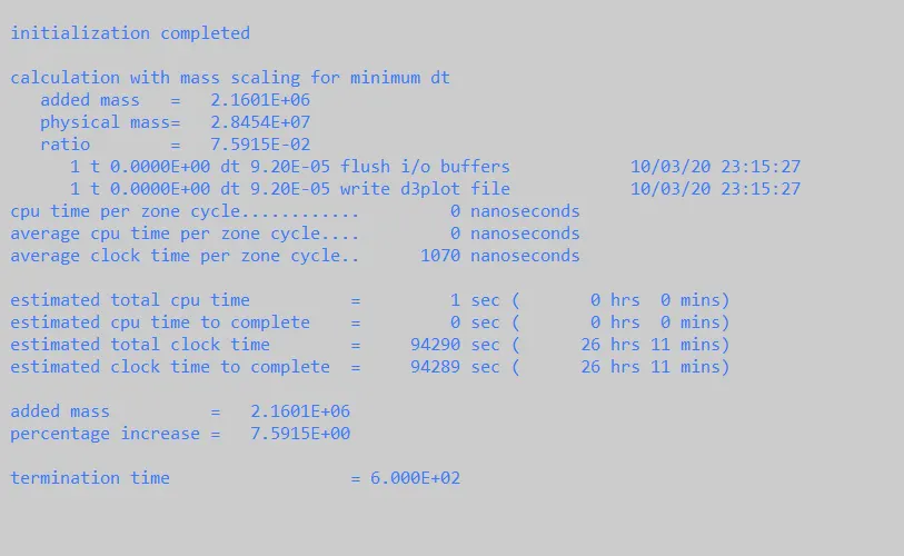
Trial 9, 

            The model have the TSSFAC and DT2MS Vaues as 0.9 and -1.023 respectively. we can see estimate the simulation time in 27hr 9mins (100440sec).

             

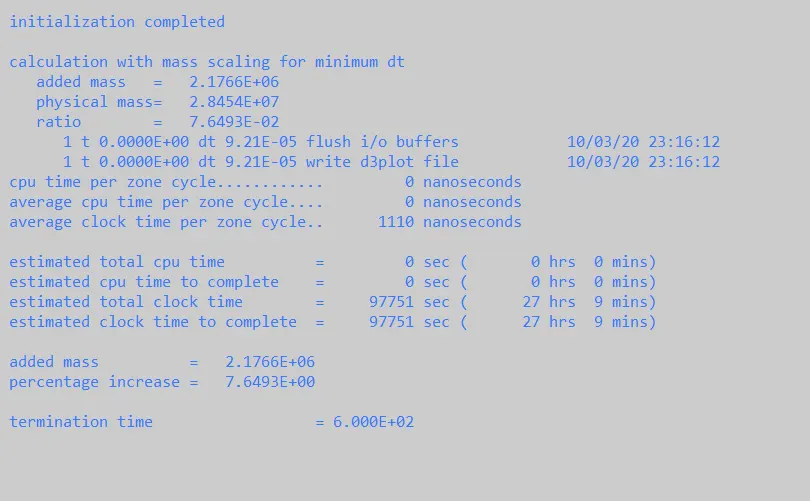
Trial 10, 

            The model have the TSSFAC and DT2MS Vaues as 0.9 and -1.024 respectively. we can see estimate the simulation time in 25hr 38mins (91368sec).

             

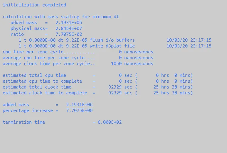
Trial 11, 

            The model have the TSSFAC and DT2MS Vaues as 0.9 and -1.026 respectively. we can see estimate the simulation time in 24hr 56mins (88416sec).

             

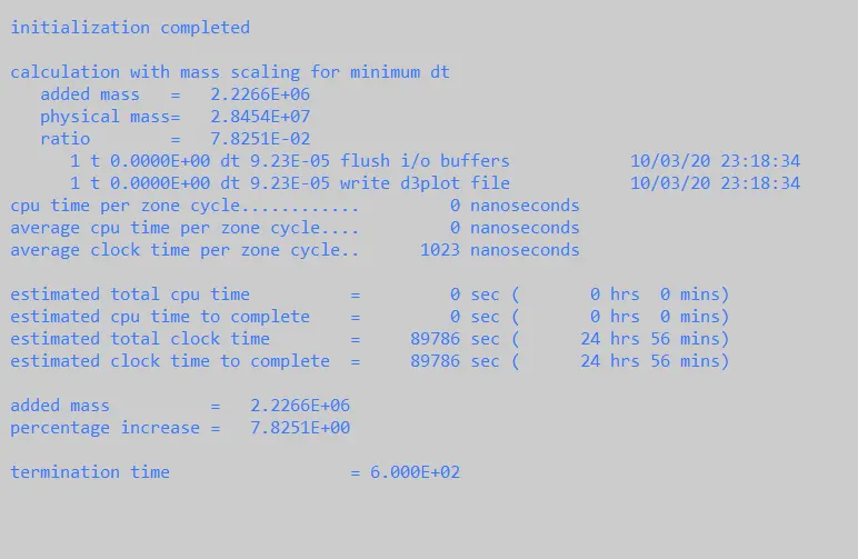
Trial 12, 

            The model have the TSSFAC and DT2MS Vaues as 0.9 and -1.028 respectively. we can see estimate the simulation time in 18hr 40mins (66240sec).

              

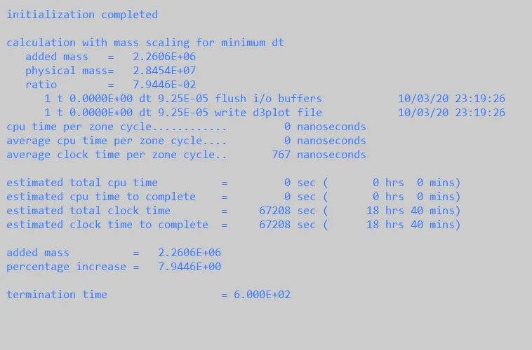
Trial 13, 

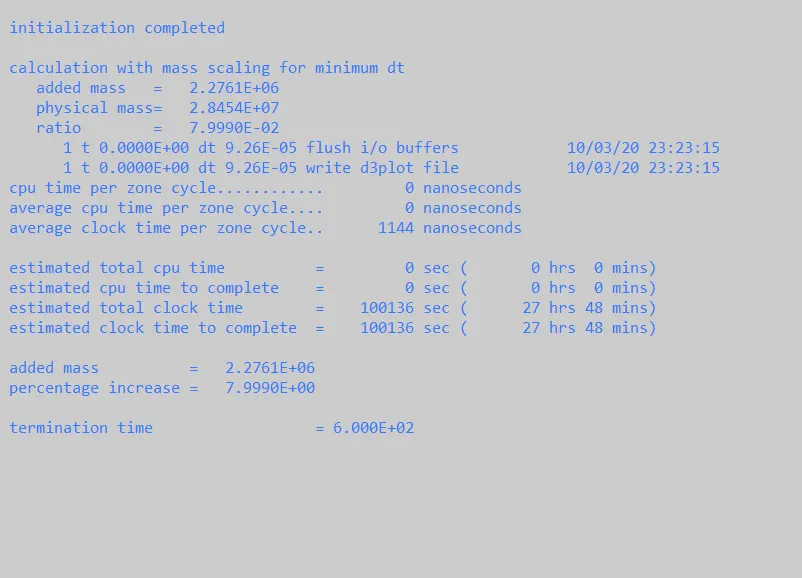
            The model have the TSSFAC and DT2MS Vaues as 0.9 and -1.0289 respectively. we can see estimate the simulation time in 27hr 48mins (98928sec).

                

Trial 14, 

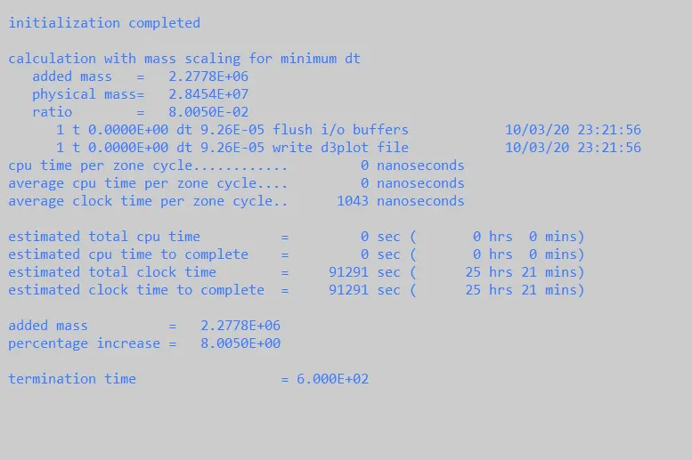
            The model have the TSSFAC and DT2MS Vaues as 0.9 and -1.029 respectively. we can see estimate the simulation time in 25hr 21mins (90756sec).

              

Histogram, 

               

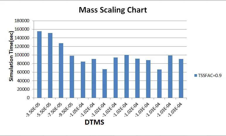
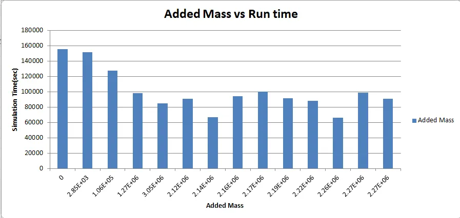
               The plot for DT2MS and the trials conducted too achieve the runtime for 8% of added mass. Further, That DT2MS conducted the element masses below the timestep level add the mass to maintain the stable condition.dont considered the above the time step. If the DT2MS values increase to step by step, simulation time is decrease certainly.

               In many cases, this two terma are used kind of interchanes ability in some case use in wrong manner. In correct way in terms of CAE analysis.

                 

Implicit Analysis,

          This model is now run with implicit method and runtime is compared with the explicit method. where the model already assign with material card and section card and also defined the stress-strain curve and mass scalling curve.

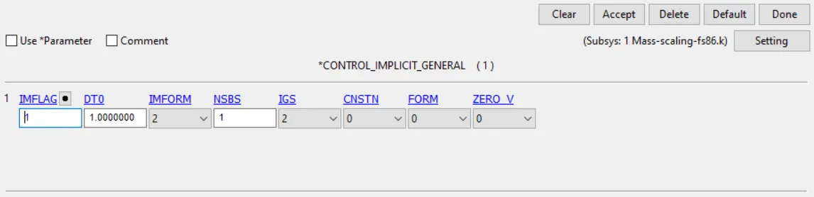
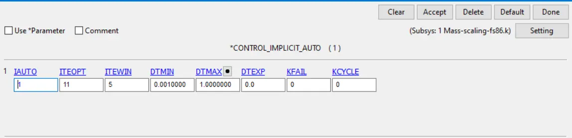
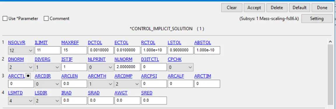
           Then, to shift from explicit to implicit analysis use the *CONTROL_IMPLICIT_GENERAL card, *CONTROL_IMPLICIT_AUTO card, *CONTROL_IMPLICIT_SOLUTION card and *CONTROL_IMPLICIT_SOLVER card.

              

              

              

Conclusion,

                From implicit method used to change the value od DT2MS values (-3.5e-5, -5.5e-6 and -7.5e-5) and simulated it. From here, if you change the mass scalling values doesn't affect the simulation time on the implicit analysis. Because, we were already assigned the simulation time and timestep also assigned on the IMPLICIT_AUTO card.

                 Time step can be controlled using the mass of the simulation. Mass scalling is only useful for the explicit simulation. And maintain the simulation and  timestep shouldn't altered slightly, its achieved by using DT2MS and TSSFAC parameters. velocity and strain rates are differenciate the implicit and explicit analysis. The explicit method should be used when the strain rates/velocity is over 10 units/second or 10 m/s respectively. These events can be best exampled by extreme scenarios such as an automotive crash, ballistic event, or even meteor impact.The implicit method should be used when the events are much slower and the effects of strain rates are minimal. Once the growth of stress as a function of strain can be established, these can be analyzed using implicit methods.