Week 8: Literature review - RANS derivation and analysis
1. AIM: To derive the Reynolds Averaged Navir Stokes(RANS) Equations and explain the following terms.
Objectives:
- To Apply reynold's decomposition to the NS equations and come up with the expression for reynold's stress.
- Explain your understanding of the terms reynold's stress
- What is turbulent viscosity? How is it different from molecular viscosity?
2. METHODOLOGY
INTRODUCTION
Fluid flow: Flow of fluid is classified into 3 types namely Laminar Flow, Transient flow and Turbulent flow. The flow is determined based on the Reynolds number.
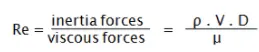
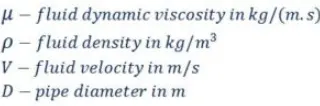
Reynolds Number: It is a measure of the ratio of inertial forces to viscous forces in a fluid flow. It is of great importance in the analysis of the boundary layer. If the Reynolds Number (based on diameter of the pipe) is less than 2100 and is turbulent if it is greater than 4000. Transitional Flow prevails between these two limits.
Formula
Whrere;
Turbulence:
Effect of Turbulence is predicted mathematically using Turbulence modelling. It is used to calculate the Reynold's stress and Turbulent Viscosity. The effect of Turbulence is modelled using Direct numerical Simulation wherein the Navier stokes equation is solved over turbulent time step.
Reynolds Averaged Navier–Stokes equations :
The Navier Stokes equations govern the velocity and pressure of a fluid flow. The velocity and pressure quantities in turbulent flow are decomposed into mean and fluctuating part. When these equations are averaged we get Reynolds Averaged Navier–Stokes equations.
Reynolds Stress: It is the component of the total stress tensor in a fluid obtained from the averaging operation over the Navier–Stokes equations to account for turbulent fluctuations in fluid momentum. The non linearity in Navier–Stokes equations means velocity fluctuations appear in RANS equations in non linear term from convective acceleration which is known as Reynolds Stress.
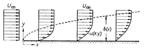
Governing Equations of Boundary Layer
Derivation:
Conservation of mass
`(delu)/(delx) +(delv)/(dely) = 0`
Conservation of momentum
`rho((delu)/(delt) +u(delu)/(delx) +v(delv)/(dely)) = -(delp)/(delx)+ mu(del^2u)/(dely^2)`
RANS decomposes flow variables into mean and fluctuating terms. The mean component is the function of space and fluctuating component is the function of space and time.
Velocity component decomposition
`u(x,y,z,t) = baru(x,y,z) + u'(x,y,z,t)`
`v(x,y,z,t) = barv(x,y,z) + v'(x,y,z,t)`
`z(x,y,z,t) = barz(x,y,z) + z'(x,y,z,t)`
Where,
`u` = Instantaneous velocity
`baru` = Average velocity
`u'` = Velocity fluctuation
The time scale is small and occur over short distance. But in Turbulence model we have to capture the effect of turbulence using courser grid and larger time step. This is achieved by taking actual governing equations and integrating them over time higher than the turbulent time scale. This process is called Averaging process. By this way Reynolds decomposition converts the original set of equations into RANS. Then we can use them along with turblence model to simulate turbulent flows.
Time Averaging: here we integrate the quanties with respect to time and do time averaging
`baru(x,y) = 1/T int_0^T u(x,y,t)dt`
`barv(x,y) = 1/T int_0^T v(x,y,t)dt`
Here`baru` is the averaging operator which is a function of x and y and does not change with respect to time
`baru = 1/T int_0^T (baru +u')dt`
`baru = 1/T int_0^T barudt +1/T int_0^T u'dt`
`baru = baru(1) + 1/T int_0^T u'dt`
Then `1/T int_0^T u'dt = 0`
Note that when we integrate the fluctuating terms for a longer period of time then fluctuation tends to zero
We can also decompose the Pressure term in the same manner
`p = barp +p'`
Substitute this decomposition into the Navier-Stokes equations and apply the time integral rule
Conservation of Mass/Continuity Equation:
`(delu)/(delx) +(delv)/(dely) = 0`
Substitute `u = baru +u'`
and `v = barv +v'`
`(del)/(delx)(baru+u') +(del)/(dely)(barv +v') = 0`
Time Averaging: here we integrate the quanties with respect to time and do time averaging
`1/T int_0^T(del)/(delx)(baru+u')dt +1/T int_0^T(del)/(dely)(barv +v')dt = 0`
`1/T int_0^T(del)/(delx)barudt +1/T int_0^T(del)/(delx)u'dt +1/T int_0^T(del)/(dely)barvdt +1/T int_0^T(del)/(dely)v'dt = 0`
Note that when we integrate the fluctuating terms for a longer period of time then fluctuation tends to zero
Then,
`1/T int_0^T(del)/(delx)barudt +1/T int_0^T(del)/(dely)barvdt = 0`
On Solving we get,
`(delbaru)/(delx)[(T-0)/T] +(delbarv)/(dely)[(T-0)/T] = 0`
`(delbaru)/(delx) +(delbarv)/(dely) = 0`
It is clear from the above equation that Reynold's decomposition satisifies continuity equation.
Conservation of Momentum :
`rho((delu)/(delt) +u(delu)/(delx) +v(delv)/(dely)) = -(delp)/(delx)+ mu(del^2u)/(dely^2)`
Multiplying `1/rho` ,we get
`(delu)/(delt) +u(delu)/(delx) +v(delv)/(dely) = -1/rho*(delp)/(delx)+ nu(del^2u)/(dely^2)`
Substituting continuity equation inside this equation.
`u((delu)/(delx) +(delv)/(dely)) = 0`
`(delu)/(delt) +u(delu)/(delx) +v(delv)/(dely) +u((delu)/(delx) +(delv)/(dely)) = -1/rho*(delp)/(delx)+ nu(del^2u)/(dely^2)`
`(delu)/(delt) +2u(delu)/(delx) +v(delv)/(dely) +u(delv)/(dely) = -1/rho*(delp)/(delx)+ nu(del^2u)/(dely^2)`
Apply Differntiation product rule
`(del(u*v))/(dely) =v(delu)/(dely) +u(delv)/(dely)`
substitue them in the equation
`(delu)/(delt) +2u(delu)/(delx) +(del(u*v))/(dely) = -1/rho*(delp)/(delx)+ nu(del^2u)/(dely^2)`
`(delu)/(delt) +(del(u^2))/(delx) +(del(u*v))/(dely) = -1/rho*(delp)/(delx)+ nu(del^2u)/(dely^2)`
As `u = baru +u'` and `v = barv +v'`
`(del)/(delt)(baru+u') +(del)/(delx)(baru+u')^2 +(del)/(dely)[(baru+u')*(barv+v')] = -1/rho*(del)/(delx)(barp+p')+ nu(del^2)/(dely^2)(baru+u')`
`(delbaru)/(delt) +(delu')/(delt) + (delbaru^2)/(delx) +(delu'^2)/(delx) + (del(2*baru*u'))/(delx) +(del(baru*barv))/(dely) +(del(baru*v'))/(dely) +(del(u'*barv))/(dely) +(del(u'*v'))/(dely)= -1/rho*(delbarp)/(delx) -1/rho*(delp')/(delx) + nu(del^2baru)/(dely^2) +nu(del^2u')/(dely^2)`
Here 2 concepts are important one is the average of square of fluctuating velocity component is not equal to zero but by considering the term is at boundary layer we can assume that variation of velcoity gradient in y direction is high in comparison to x and neglect it.
secondly when we integrate the fluctuating terms for a longer period of time then fluctuation tends to zero. Thus, by eliminating the velocity flucutation term from the above equation
`(delbaru)/(delt) + (delbaru^2)/(delx) +(delu'^2)/(delx) +(del(baru*barv))/(dely) +(del(u'*v'))/(dely)= -1/rho*(delbarp)/(delx) + nu(del^2baru)/(dely^2)`
Rearranging the equation we get
`(delbaru)/(delt) + (delbaru^2)/(delx) +(del(baru*barv))/(dely) = -1/rho*(delbarp)/(delx) + nu(del^2baru)/(dely^2) - (delu'^2)/(delx) - (del(u'*v'))/(dely)`
Neglecting `u'^2` term
`(delbaru)/(delt) + (delbaru^2)/(delx) +(del(baru*barv))/(dely) = -1/rho*(delbarp)/(delx) + nu(del^2baru)/(dely^2) - (del(u'*v'))/(dely)`
`(delbaru)/(delt) + (delbaru^2)/(delx) +(del(baru*barv))/(dely) = -1/rho*(delbarp)/(delx) + 1/rho(del)/(dely)(mu(delbaru)/(dely) - rho*u'*v')`
Unsteady Reynolds Average N-S equation :
`rho((delbaru)/(delt) + (delbaru^2)/(delx) +(del(baru*barv))/(dely)) = -(delbarp)/(delx) + (del)/(dely)(mu(delbaru)/(dely) ubrace(- rho*u'*v')_(Reynolds Stress))`
In the above equation `rho*u'*v'` represents Reynold's stress on the fluid.
Reynolds Stress: It is the component of the total stress tensor in a fluid obtained from the averaging operation over the Navier–Stokes equations to account for turbulent fluctuations in fluid momentum. The non linearity in Navier–Stokes equations means velocity fluctuations appear in RANS equations in non linear term from convective acceleration which is known as Reynolds Stress.
Formulae:
`tau'_(uv) =-rho*u'*v'`
In turbulent flow Reynold stresses are large compared to Viscous stresses. It provides the averaged effect of turbulence which is highly diffusive and the normal stresses are always zero as they contain only squared velocity fluctuations.
What is turbulent viscosity? How is it different from molecular viscosity?
Turbulent Viscosity assumes that the Reynolds stresses can be related to mean velocity gradients and turblent viscosity by gradient diffusion hypothesis. Turbulent viscosity is not homogeneous ie., it varies in space but isentropic.
It is also known as eddy Viscosity since linear interface between the different fluids breaks apart to form slim scale structures called eddies. They diminish as they grow and alter the surface area of the interface between the fluids with various properties by altering the net heat transfer of momentum and scalar properties through the interfaces.
Molecular Viscosity is the resistance to the movement of one layer of fluid ove the adjacent layer. It is linear, easy to measure quantity and independent of geometry. The coefficient of molecular viscosity is same as dynamic viscosity. It is the transport of mass motion momentum soley by the random motions of individual molecules not moving together in coherent groups. It is analogous in laminar flow to eddy viscosity in turbulent flow.
Finally,
Turbulent viscosity is imaginary and molecular viscosity is dynamic viscosity present in real fluids.
Molecular viscosity depends on properties of fluid and turbulent viscosity depends on the fluid flow.
Molecular viscosity is dominant in regions of low reynold's number and turbulent viscosity is dominant in regions of high reynold's number.
3. CONCLUSION
Reynold's stress expression was derived by using Reynold's decomposition to Naviers Stokes equation and theory behind Molecular viscosity, Turbulent viscosity and Reynold's stress was also studied.