Week 8: Literature review - RANS derivation and analysis

Reynolds- Averaged Navier Stokes(RANS) equation

RANS equations are time-averaged equations governing the motion of fluid flow. The methodology of reynold's decomposition, wherein an instantaneous property is decomposed into mean or time-avergaged and fluctuating components, is used to approximate the NS equations. RANS equations are primarily used to describe turbulent fluid flows.

1. Governing equations for a boundary layer

For a 2D incompressible fluid, by performing order of analysis on the Navier Stokes equation, the equations can be simplified as follows:

1.1 Continuity equation

`(delu)/(delx) + (delv)/(dely) = 0`

1.2 Momentum equation

`rho ( (delu)/(delt) + u(delu)/(delx)+v(delu)/(dely)) = -(dP)/dx + mu((del^2u)/(dely^2))`

1.3 Energy equation

`rho_c((delT)/(delx)+u(delT)/(delx)+v(delT)/(dely))=k(del^2T)/(delx^2) + mu((delu)/(dely))^2`

The above set of equations can be solved without using a turbulent model, a technique called as direct numerical solution. However, it is to be noted that the velocity fluctuations occuring in a point in the boundary layer has very high frequency and the associated turbulent timescale is very small. Thus, the computational mesh must be very fine (in the order of microns) and the total computational cells must be very large. This prospect makes the simulation extremely slow and expensive.

To improve the simulation time and adopt coarser mesh to capture the turbulence characteristics, we perform reynold's decomposition on the given set of governing equations

2. Reynold's decomposition

It involves decomposing a flow characteristic variable into a mean componet and fluctuating component. For example, the instantanteous velocity along x-direction can be written as:

`u(x,y,z,t) = bar u(x,y,z)+u'(x,y,z,t)`

where `bar u` represents the time-averaged mean component and u' represents the fluctuating component.

Also, by definition,

`bar u(x,y,z) = 1/t_"int"int_0^(t_"int")u(x,y,z,t).dt` ....(1)

Note- The mean component is time-averaged and hence, it is not dependent on the time of simulation.

2.1 Time integral of fluctuating component

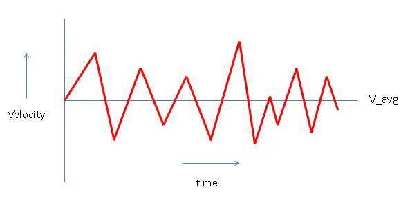
Consider a fluctuating velocity as shown in the figure above. When the time-scale of simulation is large, the area of the curve above the mean is equal to that below the mean. That is, the integral of the fluctuation over the time scale is zero.

`int_0^(t_"int")u'(x,y,z,t).dt = 0`

Another way to prove this is by integrating the flow characteristic

`u(x,y,z,t) = bar u(x,y,z)+u'(x,y,z,t)`

`1/t_"int"int_0^(t_"int")u(x,y,z,t).dt = 1/t_"int"int_0^(t_"int")bar u(x,y,z).dt + 1/t_"int"int_0^(t_"int")u'(x,y,z,t).dt`

We know that the integral of a mean function is the mean function itself. Using this and from (1), we can rewrite this as:

`bar u(x,y,z) = bar u(x,y,z) + 1/t_"int"int_0^(t_"int")u'(x,y,z,t).dt`

Therefore,

`int_0^(t_"int")u'(x,y,z,t).dt = 0` ...(2)

2.2 Simplication of the NS equations

2.2.1 Reynolds decomposition of continuity equation

`(delu)/(delx) + (delv)/(dely) = 0`

`(del(bar u + u'))/(delx) + (del(bar v+v'))/(dely) = 0`

Integrating on both sides,

`1/t_"int"int_0^(t_"int")(delbar u)/(delx) +1/t_"int"int_0^(t_"int")(del u')/(delx)+1/t_"int"int_0^(t_"int")(delbar v)/(dely)+1/t_"int"int_0^(t_"int")(delv')/(dely) = 0`

Taking derivatives common from the terms,

`(del/(delx))(1/t_"int"int_0^(t_"int")(bar u + u').dt) + (del/(dely))(1/t_"int"int_0^(t_"int")(bar v + v').dt) =0`

From (2), we get

`(delbar u)/(delx) + (del barv)/(dely) = 0`

2.2.2 Reynolds decomposition of momentum equation

`(delu)/(delt) + u(delu)/(delx)+v(delu)/(dely) = -(1/ rho)(dP)/dx + (mu/rho)((del^2u)/(dely^2))` ...[I]

Now, based on the continuity equation,

`u((delu)/(delx) + (delv)/(dely)) = 0` ...[II]

Adding [II] to [I], we get

`(delu)/(delt) + u(delu)/(delx)+v(delu)/(dely) + u((delu)/(delx) + (delv)/(dely)) = -(1/ rho)(dP)/dx + (mu/rho)((del^2u)/(dely^2))`

`(delu)/(delt) + 2*u(delu)/(delx)+v(delu)/(dely) + u (delv)/(dely) = -(1/ rho)(dP)/dx + (mu/rho)((del^2u)/(dely^2))`

Using product rule of integration,

`(delu)/(delt) + (del(u^2))/(delx)+(del(uv))/(dely) = -(1/ rho)(dP)/dx + (mu/rho)((del^2u)/(dely^2))`

Integrating on both sides and applying reynolds decomposition,

`1/t_"int"int_0^(t_"int")[(del(baru+u'))/(delt) + (del((baru+u')^2))/(delx)+(del((baru+u')(barv+v')))/(dely)].dt =1/t_"int"int_0^(t_"int")[ -(1/ rho)(d(barP+P'))/dx + (mu/rho)((del^2(baru+u'))/(dely^2))].dt`

By eliminating the fluctuating components, we can simplify the equation as

`1/t_"int"int_0^(t_"int")[(delbaru)/(delt) + (delbaru^2)/(delx)+(delu'^2)/(delx)+(del(barubarv))/(dely)+(delu'v')/(dely)].dt =1/t_"int"int_0^(t_"int")[ -(1/ rho)(dbarP)/dx + (mu/rho)((del^2baru)/(dely^2))].dt`

Therefore, by evaluating the mean integral terms,

`(delbaru)/(delt) + (delbaru^2)/(delx)+(del(barubarv))/(dely)+1/t_"int"int_0^(t_"int")(delu'^2)/(delx).dt+1/t_"int"int_0^(t_"int")(delu'v')/(dely).dt = -(1/ rho)(dbarP)/dx + (mu/rho)((del^2baru)/(dely^2))`

Comparing this equation with the momentum equation, we find the additional terms are

`1/t_"int"int_0^(t_"int")(delu'^2)/(delx).dt+1/t_"int"int_0^(t_"int")(delu'v')/(dely).dt`

As the boundary layer thickness is very small compared to the characteristic length of the fluid domain, the square of the fluctuations can be neglected. That is,

`1/t_"int"int_0^(t_"int")(delu'^2)/(delx).dt =0`

Rewriting the decomposed momentum equation,

`(delbaru)/(delt) + (delbaru^2)/(delx)+(del(barubarv))/(dely) = -(1/ rho)(dbarP)/dx + (mu/rho)((del^2baru)/(dely^2))-1/t_"int"int_0^(t_"int")(delu'v')/(dely).dt`

`(delbaru)/(delt) + (delbaru^2)/(delx)+(del(barubarv))/(dely) = -(1/ rho)(dbarP)/dx + (1/rho)(del/(dely))[(mu(delbaru)/(dely))-rho/t_"int"int_0^(t_"int")(u'v').dt]`

3. Reynolds averaged Navier's Stokes equation

`ubrace((delbaru)/(delt) + (delbaru^2)/(delx)+(del(barubarv))/(dely))_("Inertial terms") =ubrace( -(1/ rho)(dbarP)/dx)_("Pressure terms") + ubrace((1/rho)(del/(dely))[(mu(delbaru)/(dely))-rho/t_"int"int_0^(t_"int")(u'v').dt])_"Momentum diffusivity terms"`

We can denote the terms in the reynolds decomposed NS equations as interial terms, pressure term and the momentum diffusivity term. This momentum diffusivity is modelled using a turbulence models. The momentun diffusivity terms can be further classified as:

`ubrace((mu(delbaru)/(dely)))_"viscous stress"-ubrace(rho/t_"int"int_0^(t_"int")(u'v').dt)_"reynolds stress"`

3.1 Viscous stress and associated molecular viscosity

On comparing the first term with the characteristic equation of a Newtonian fluid, we can say that `mu(delbaru)/(dely)` represents the viscous stress inside the boundary layer. The associated viscosity is due to the molecular viscosity `mu`

3.2 Reynolds stress and associated turbulent viscosity

The term `rho/t_"int"int_0^(t_"int")(u'v').dt` is defined as the reynolds stress. This is developed due to the fluctuation in the horizontal and vertical velocities and the associated viscosity is termed as the turbulent viscosity.

Reynolds stress results from turbulence diffusivity of momentum. It is the component of total stress tensor obtained by time-averaging the NS equations and accounts for the turbulent fluctuations in fluid momentum.

Turbulent viscosity, also known as eddy viscosity, is due to the turbulent fluctuations in the velocity components of fluid flow. The turbulent transfer of momentum by eddies giving rise to an internal fluid friction, in a manner analogous to the action of molecular viscosity in laminar flow, but taking place on a much larger scale. However, unlike the molecular viscosity, the turbulent viscosity is a flow parameter and is not a property of the system. That is, the molecular viscosity is dependent on the type of fluid, pressure and temperature conditions. But the turbulent viscosity is only dependent on the flow parameters such as Reynolds numberof fluid flow.