Week 7 State of charge estimation

In coulomb counting method, we continuously count the charge which has left or entered the cell to keep track of remaining charge. This is done through instantaneous measurements of current and time. It can be understood by analogy of water entering/leaving a tank. If water enters/leaves tank at the speed of y cu. metre/second for 10 seconds, then total water added/left will be 10y cu. metre (simply, flow rate x time). In case of electrons, flow rate is current and thus charge left/entered will be current x time. Since, the current will vary, hence instantaneous measurements are taken, thus

inst. change in charge = current x inst. time

Integrating both sides we get,

Total change in charge = `int`Idt

Final Ah = Initial Ah + Change in charge = Initial Ah + `int`Idt

(where I>0 during charging and I<0 during discharging)

This algorithm, is continuously run in an infinite loop of a microprocessor/microcontroller. The high clock speed of microcontroller allows it to very accurately measure the change in SOC. Change in SOC at every iteration of infinite loop is calculated as function of product of instantaneous current and sample time. This change in SOC is added/subtracted to present value of SOC to get new value of SOC as shown in image below -

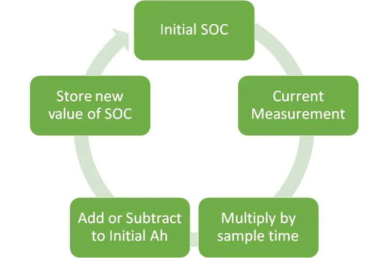
But this method faces, Convergence Issue. The coulumb counting method relies on the current measurement measured from voltage drop across the shunt resistor. This shunt resistor measurement accuracy is dependent on various parameters such as shunt resistor tolerance, ambient temperature, temperature due to current, quality of Analog-to-digital converter on microprocessor. This error in current reading accumulates over time and causes a divergence between the calculated and real SOC. Thus, this method is usually used in conjunction with other methods for better accuracy.