Week 7 State of charge estimation

Aim :-

1.Simulate the 3 test cases from harness dashboard and write a detailed report on the results

2.What is coulomb counting? Refer to the above model and explain how BMS implements coulomb counting for SOC estimation ?

Explanation :-

In file exchange open the document of Design and Test Li-ion battery management algorithm.

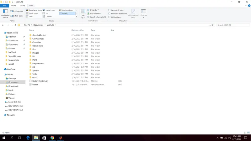
Download the zip files and extract to a folder, the folder consist of these files as shown below.

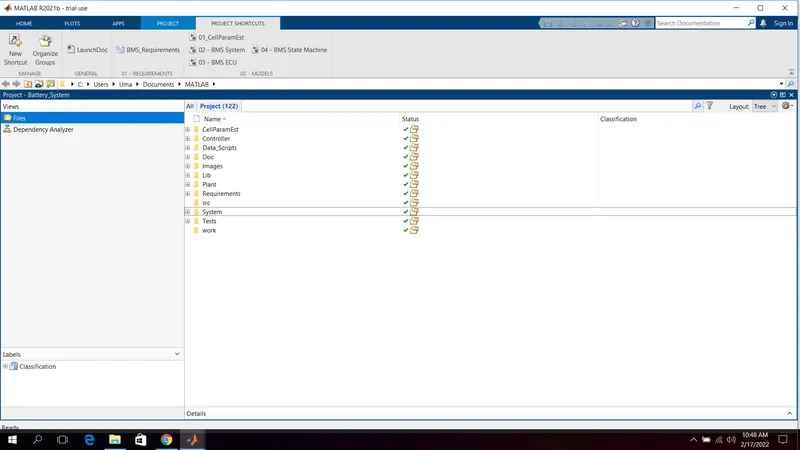
Open Matlab software and open the simulink model file closed loop BMS harness dashboard in tests.system..BMS..Closedloop..Harness..Dashboard model file.

The give open project and model and model in pop-up-dialogue box to install all the model related library files into the current folders and workspace.

The model file open as,

Model Explanation :-

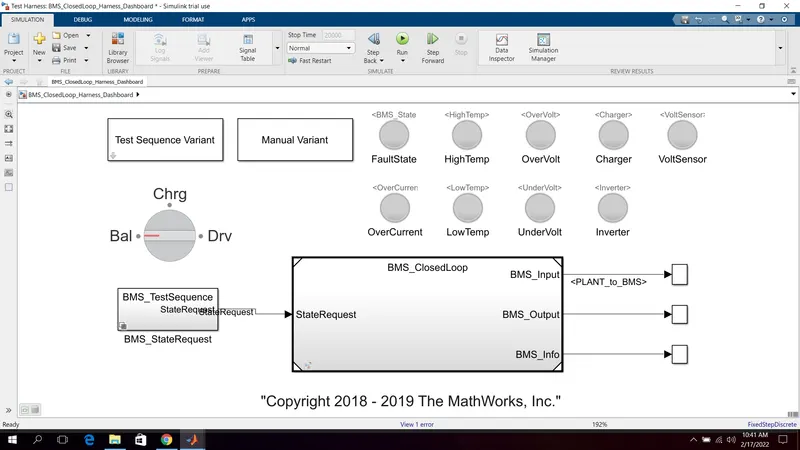
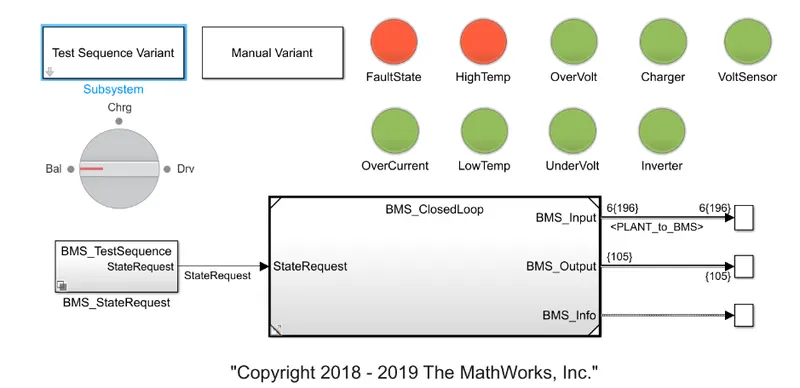
1.DashBoard :-

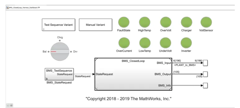
1. Test sequence varient.

2. Manual varient.

3. BMS_Test sequence state request to provide state request commands.

4. Lamps to indicate fault state, high temperature, over voltage, over current, charging voltage, sensor opertion, inverter operation, low temperature, under voltage. If any fault in these red indication will intimate us and all in good conditions indicated will intimate us and all in good conditions indicated by green indication.

5.Rotating switch for manual varient changes while running simulation.

6. In scope results the SOC of module, Module current, individual cell voltage, individual cell temperature battery state cell balancing states are seen as outputs.

2.BMS_Closed Loop :-

In this main block consist of two subsystem BMS ECU and PLANT units.

The plant output from plant unit given as input to BMS ECU as BMS_input feedback loop, the state request is given to BMS ECU unit.

The BMS output commands given as input to plant unit as From_BMS, the state request is given to plant unit.

The final outputs from closed loop model are BMS_input, BMS_output, BMS_info.

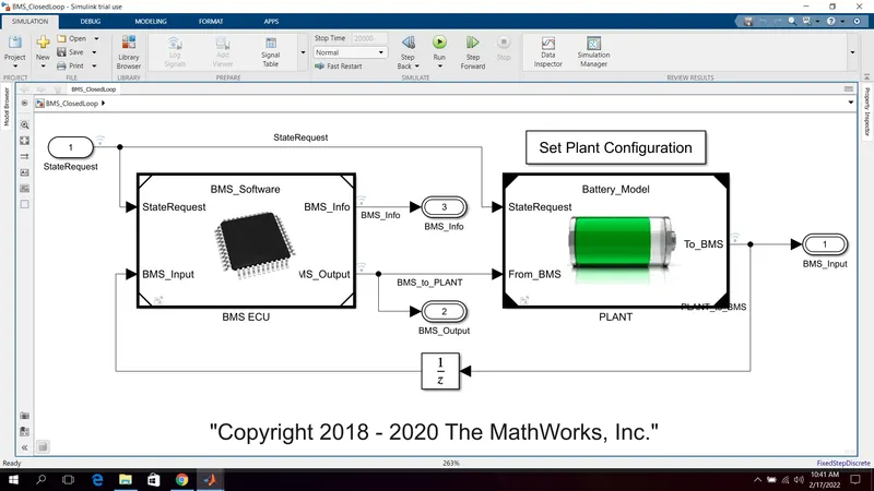
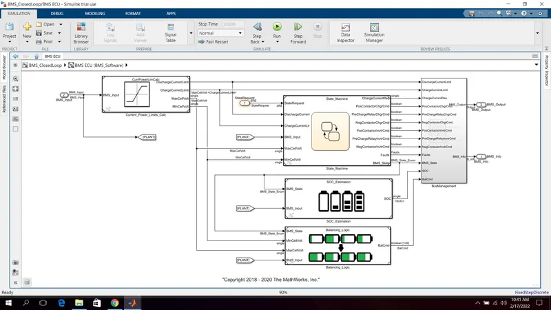
In BMS ECU unit the current power limit calculations are done used in state machine block, Soc estimations cell balancing logics as shown below.

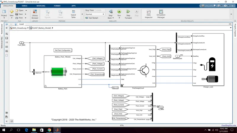
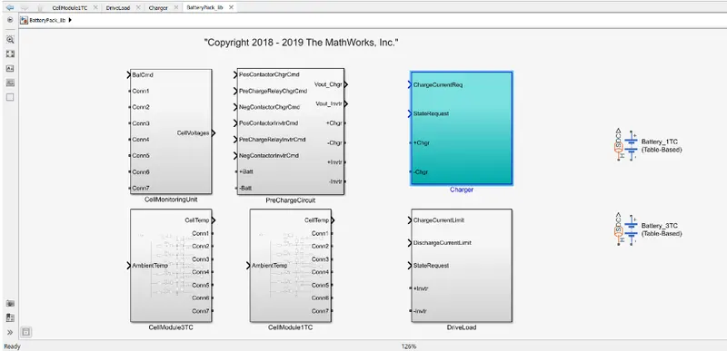
In plant unit the battery pack unit, pre charge unit charger/load units are created.

In battery pack there are two types of configuration as 1 module 6 cells and 16 modules 95 cells.

Here we are closing 1 module for lesser simulation running time.

A). To run three test cases from harness dashboard of closed loop BMS control;

We have to test three cases for this model by selecting test sequence varient and select the cases one by one as follows,

Test case 1:

Select 1 from test sequence varient dialog box and click apply as shown below.

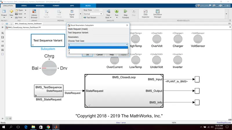
This selection consist of selection changes in masked BMS_State request subsytem as,

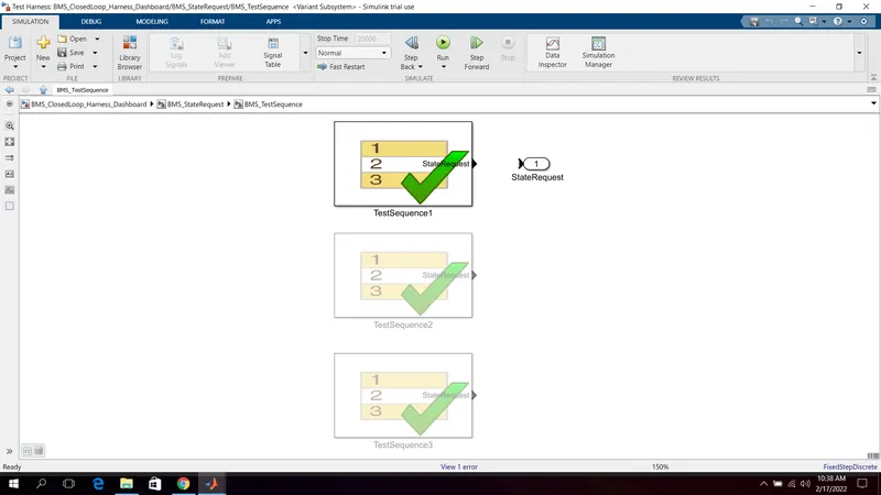
This test case consist of the following sequence operation as,

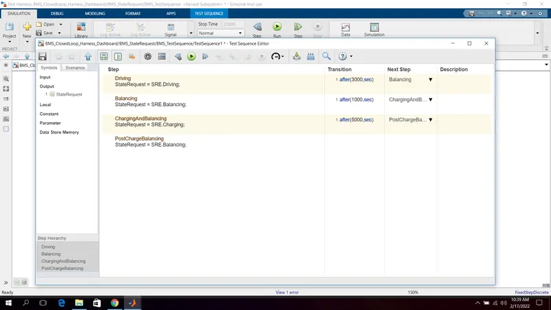
Here from the above test sequence editor figure it was set as,

1. Driving for first 3000 secs.

2. After 3000 sec starts balancing operations occur for next 1000 secs.

3. Then charging and balancing occurs for next 5000 secs.

4. After that sequence post charge balancing operation occurs till end of the simulation period.

Output :-

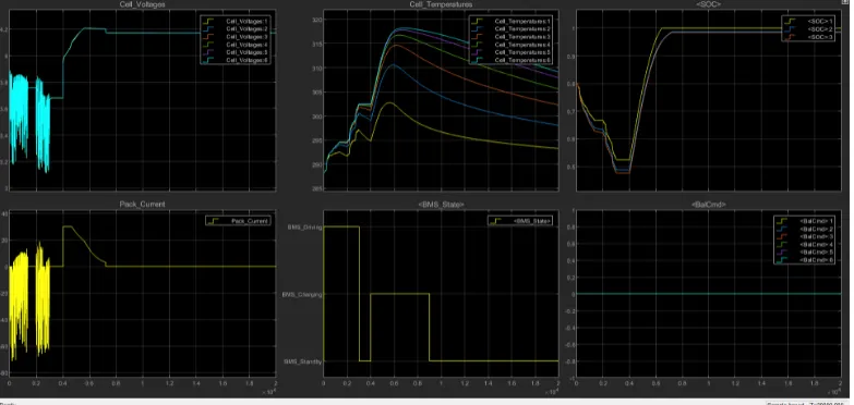
Run the simulation land results are shown as.

The lamp indications are showing green for overall simulation period showing that there are no faults occurs during the sequence.

From the results we can understand that,

Cell Voltage and Pack Current :-

For first 3000 secs all 6 cells are drive model where discharging occur majorly and in standby mode for lesser duration at approximately 1000 to 2000 secs.

The voltage varies from 3.1V to 3.9V in this range. From 3000 sec to 4000 sec cell balancing occur and this stage the module in standby mode and voltage in constant nearly 3.7V.

After 4000sec charging occur voltage raised from 3.7V to 4V at 4V to 4.2V constant current as nearly 30A after 4.2V constant voltage current reduce from 30A to 2.6A.

At end of the charging and cell balancing occurs upto 9000sec. After 9000 sec post charge cell balancing starts. All cell voltage are balancing to a voltage with respect to cell 1 to 4.1V shown.

Cell Temperature :-

Initially for 3000sec the temperature range of cells increase gradually from ambient temperature 288k to 302k.

The temperature of cell is lesser and cell 6 has higher temperature for all stages. After 4000sec temperature start increase exponentially upto constant current region and start reduces as current flow reduces in constant voltage and cell balancing region upto 9000sec.

Cell 1 max temperature raised upto 302k and cell 6 temperature raised upto 317k. After 9000sec the temperature still reduce and remains stable at reaching ambient temperature.

BMS State :-

For 3000sec the battery module in drive mode.

From 3000sec to 4000sec the battery module in balancing standby mode as shown.

After 4000sec upto 9000sec the battery module in charging and balancing mode.

After 9000sec only post charge balancing mode operates upto end of simulation.

SOC :-

Initially the state of charge of battery module is in 80%. Here the yellow plot represent SOC estimation done by coulomb counting technique.

Blue plot represents SOC estimation using unscented kalman filter technique. Red plot represents SOC estimation using extended kalman filter technique, among three UKF and EKF technique estimate accurately than coulomb counting technique.

Initially for 3000sec SOC decreases to nearly 45% during drive mode. After 3000sec upto 4000sec the SOC is constant at 45% cell balancing occur in standby mode.

From 4000sec to 9000sec module in charging mode. After 9000sec the SOC between constant approximately 94% as seen from above plots.

Balancing Cells :-

Initially upto 3000sec balancing was not performing. After 3000sec cell balancing starts with on cell 6 and cell 2 as they rised to as shown . After this stage charging and balancing post charge balancing are occur as cell 6 and cell 2 remian in 1 state sill end of simulation.

As cell is in lesser voltage than other cells it remains in 0 state through out the simulation. At the end of the simulation all cell votlage try to balance equally as we seen earlier in signal cell votlage plot.

Test Case 2 :-

Now select test case 2 and click apply in test sequence varient dialog box shown;

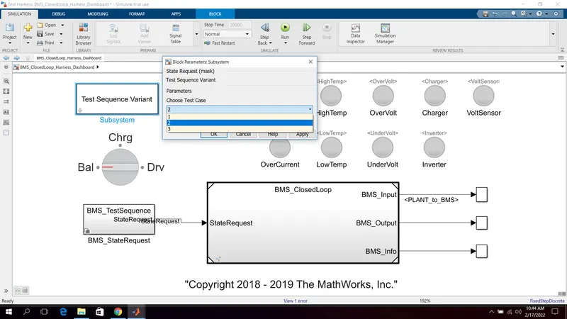
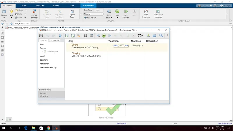
The case altered to second shown,

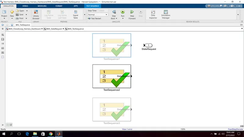
This test case constist of drive mode for 10000sec and after that charging occur till end of simulation.

Now run the model and result can be viewed.

Output :-

Dashboard reults are shown,

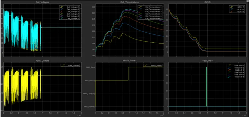
The scope result plotted as,

Cell Voltage and Pack Current :-

The cell voltage varies from maximum 3.9V and reduce to 3.05V as cutoff voltage upto 9000sec entire capacity drained at 9000sec. The pack current discharge upto maximum 70A and slight charging occur during the over all drive.

Some stand by mode conditions are in between the drive mode.

Cell Temperature :-

Here cell 1 lesser temperature variation from 288k to approximately 302.5k. Cell 6 in haivng temperature variation from 288k to approximately 322.5k. The cell temperature are slightly reducing in between drive mode as these duration are in stand by.

Battery Module State :-

Entire sequence is performing in drive mode as shown the plot. Small duration of standby modes are not ploted in this plot a simulation 10000sec command is given as drive mode.

But in acutal practival situation stand by modes are not present battery current drains by other small of EV's.

SOC of module :-

Here the SOC reduce from 80% to 0% in entire drive mode as shown above plot. At stand by modes in between them the SOC remians constatn as shown.

Balancing :-

Here balancing of cells are not performed as shown as balance states are in 0 for entire drive mode.

Test Case 3 :-

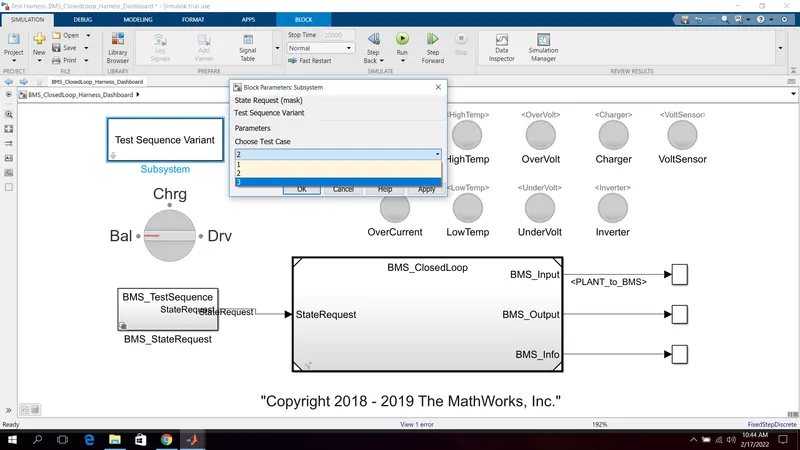
Now select test case 3 click apply in test sequence varient dialog box as shown below,

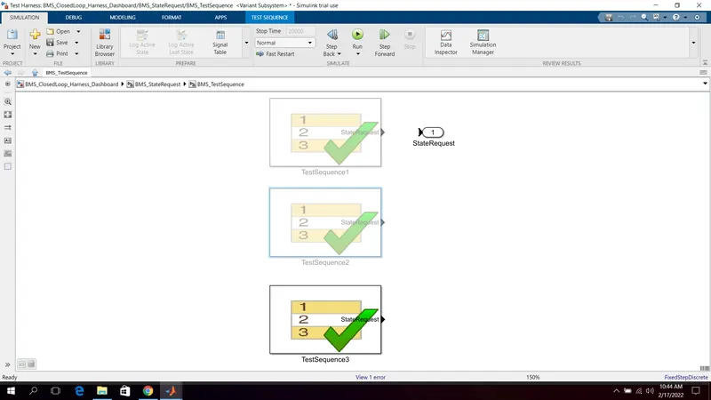
The test case is altered to third as shown,

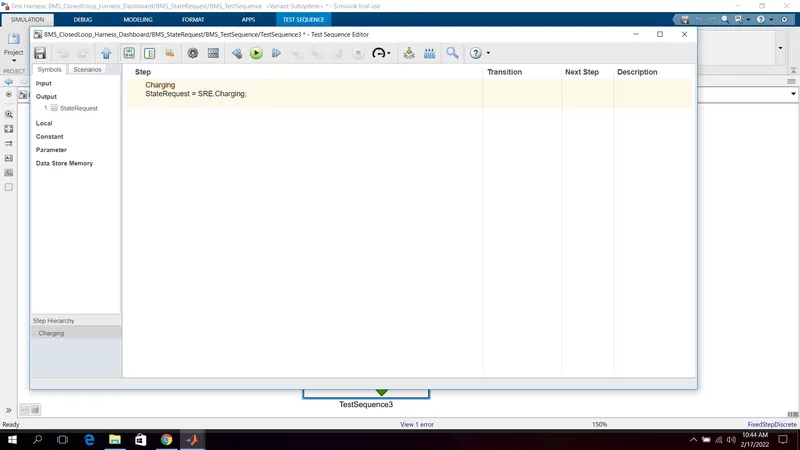
This test case consist of charging for entire duration of time.

Run the model and results can be viewed.

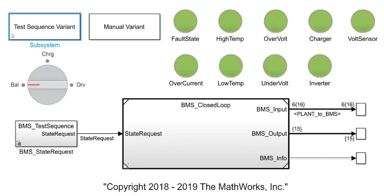
All indicarion are in green indicate no fault conditions are occur,

The plots are shown as,

Cell voltage and pack current :-

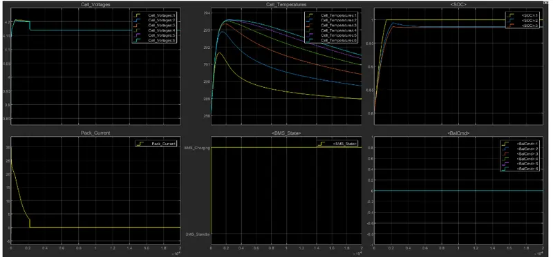
Initially cell 2 voltage rises from 3.9V to maximum 4.2V and stabilised to 4.15V. Cell 1 rises form 3.85V to 4.1V and stabilised to 4.08V.

The battery pack current raising form 0A to 30A and start to reduce to 2.5A gradually at end to full charging 2000sec. After full charge current flow will be cutoff as show in result plot.

Cell Temperature :-

Cell Voltages and Pack Current :-

Initially cell 2, voltage rises from 3.9V to maximum 4.2V and stabilised to 4.15V.

Cell 1 rises from 3.85V to 4.1V and stabilised to 4.08V.

The battery pack current raising from 0A to 30A and start to reduce to 2.5A gradually at end to full charging upto 2000 secs.

At 2000 secs the pack is fully charged to 100%.

After full charge current flow will be cutoff as shown in result plot.

Cell Temperatures :-

The cell temperature continue to increase heat upto full charge and after that the temperatures get started to reduce to ambient temperature.

As shown from result plot the temperature start decreases after full charger.

BMS State :-

Entire battery pack sequence is operating in charging mode as shown above.

SOC :-

The pack SOC gets fully charged at 2000sec and remians at full charge for rest of the sequence as shown above.

The actual state of charge is around 93% shown as full charge shown by UKF and EKF techniques.

Cell Balancing :-

Here form 0sec the cell 6 and 2 starts to balance with respect to cell 1 and all cells are try to balancing at end of simulation.

Hence from above three test cases the performance of BMS on various factors are discussed and analysed.

B) To explain coulomb counting for finding the SOC estimation in BMS;

Coulomb counting :-

SOC is defined as the rate of available capacity to its maximum capacity when a battery is fully charged and describes the remaining percentage of the battery.

To find this SOC we are using coulomb counting method.

The coulomb counting method measures the discharging current of the battery and integrates the discharging current over time in order tp estimate SOC.

Which can be estimated from discharging current , previously estimated SOC values,

SOC(t) = SOC(t - 1) + (I(t)/Qn)delta(t).

Modified Coulomb counting :-

In this technique discharge current is connected with a function and corrected current is found out for accurate SOC estimation.

Ic(t) = k2I(t)^2 + k1I(t) + k0,

where k0,k1,k2 are constant values obtained from the practice experimental data.

The SOC relation can be given,'

SOC(t) = SOC(t -1 ) + (Ic(t)/Qn)delta(t).

SOC estimation in BMS model :-

To see model of coulomb counting technique in BMS model click the subsytem of SOC_estimation and click coulomb counting.

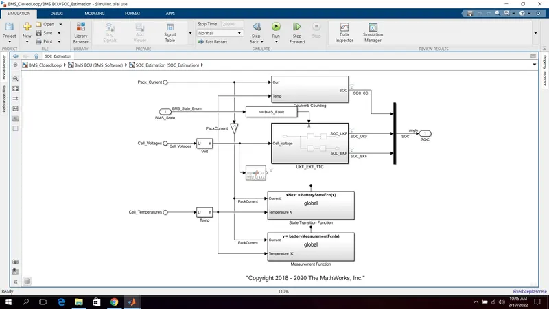
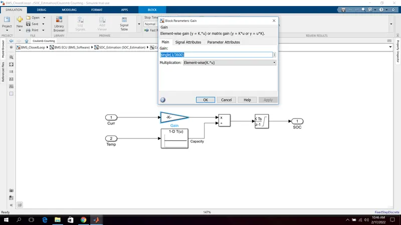
Here the discharge current from battery given to gain with value as 1/3600 to convert current to Ahr.

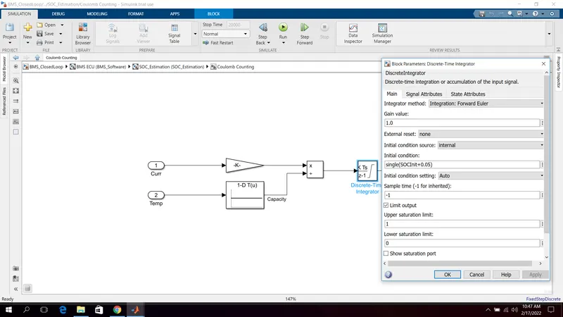
The value is divided by capacity due to temperature change. Then integrated with a gain value of 1 with sample time-1 as we are using discrete integrator.

We will get the SOC value from 0 to 1 multiple with 100 to get in percentage of SOC.

Conclusion :-

Simulate the 3 test cases from harness dashboard and write a detailed report on the results. Refer to the above model and explain how BMS implements coulomb counting for SOC estimation are explained clearly and successfully.