State of Charge Estimation Using MATLAB

Understanding SOC Estimation Using MATLAB & Simulink

Aim -

• To Simulate 3 test cases from the harness dashboard and write a detailed report on the result
• To write a detailed report on the Coulomb counting method.

Model Used - https://in.mathworks.com/matlabcentral/fileexchange/72865-design-and-test-lithium-ion-battery-management-algorithms

Tools Used - MATLAB Simulink Workbench

Simulink Model -

• BMS_Closed loop model -

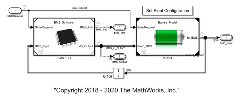
• The BMS_Closedloop model consists of 2 major Subsystems, BMS ECU and Battery plant.
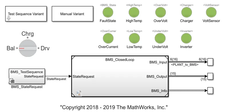
• The Output from the BMS ECU subsystem is provided as input in the Plant subsystem through From BMS port. Also, state requests are also provided to both the subsystems.
• The Plant output is also provided into the BMS ECU subsystem in a closed-loop format.

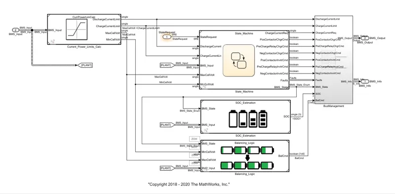
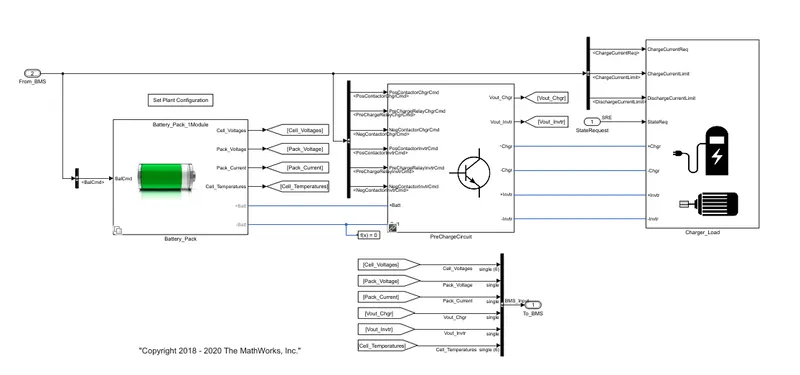
Subsystem Layouts -

Test Case - 1

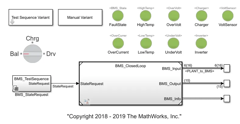
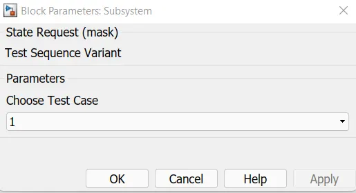
Select test sequence 1 from the Test sequence variant block.

Test Sequence Data for test case 1

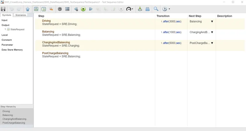
• According to test sequence case, 1 data the simulation will simulate the driving case for 3000 sec followed by balancing of cells for 1000 sec and Charging and balancing for next 5000 sec.
• Post charging Balancing is done for the rest of the simulation.
• The total run time for the simulation is 20000.

Results -

Cell Voltage and Pack Current -

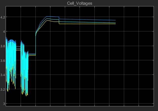
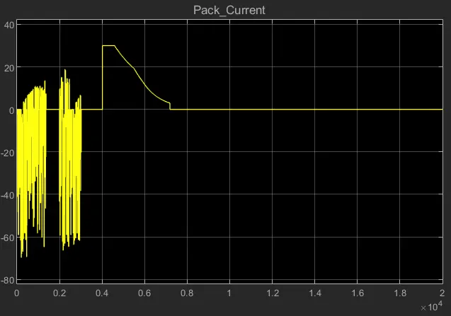
• During Driving Cycle Simulation the cell voltages vary between 3.1 to 3.9 V
• During Cell balancing the Voltage remains constant at around 3.7 Volts.
• After 4000 Sec the charging phase initiates the cell voltage rise from 3.7 to 4V and then to 4.2 V, The current is constant 30 A, and after that, it is reduced to 2A current gradually and is kept constant.

Cell Temperature -

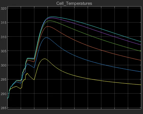
• From 0 to 3000 sec the cell temperature rises from 288 K to up to 302 k maximum.
• The temperature of cell 1 is lower as compared to that of cell 6
• From 3000 sec to 4000 sec the temperature remains constant as no current is flowing through the cell.
• The temperature starts rising from t = 4000 sec and continues to rise up to the constant current region and then starts to reduce exponentially.

BMS Mode -

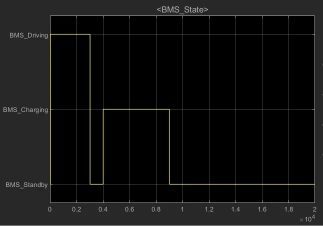
• The BMS is in driving mode for 3000 sec
• From 3000 to 4000 Sec it is on standby mode
• From 4000 to 9000 it is in charging mode and for the rest of the simulation it is again in standby mode

SOC -

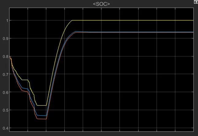
• The initial state of charge is at 80%
• Yellow - Columb counting method
• Blue - Unscented Kelman method
• Red - Extended Kalman filter method
• Initially, the SOC is dropped to 45 % during driving and remains constant during cell balancing as it is happening in a standby period. During charging the SOC is increased gradually charged to 94%.

BMS -

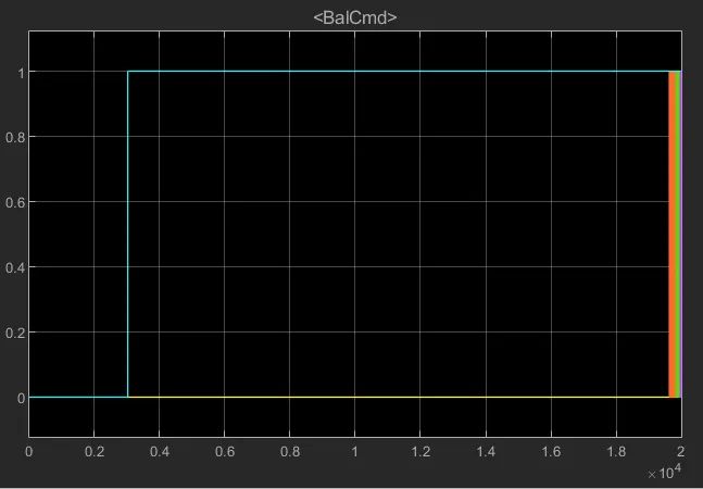
• The cell balancing starts at 3000 sec, Cell 2 and 6 are balanced initially while the rest of the pack starts balancing during the end of the simulation.

CASE - II

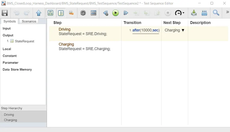
• In this case, the simulation is only Simulates the Driving and Charging cycle. The transition will happen after 10000 sec and the simulation time is 20000 sec.

Results -

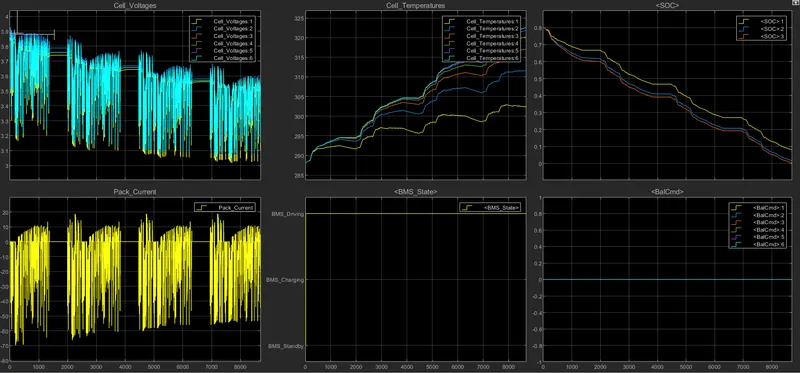
Cell Voltage and Pack Current -

• The Cell Voltage Varies between 3.9 to 3.05 V which is the cut-off value.
• The cell reaches the cut-off value in 9000 sec.
• The maximum current drawn is 70Ampere from the battery pack.

Temperature -

• The temperature of the cells varies between 302 to 322 k maximum.
• Cell 6 has attained maximum temperature among all the cells in the battery pack.

SOC -

• The Initial SOC of the battery pack is at 80 %
• 3 modes of SOC calculation are used Colomb counting(yellow), Unscented Kalman method(blue), and Extended Kalman filter(red) method. The latter 2 are more accurate than the coulomb counting method.
• The SOC of the battery is down to 0% at the 9000 sec of the Simulation.

In this Case balancing of the battery is not done.

CASE - III

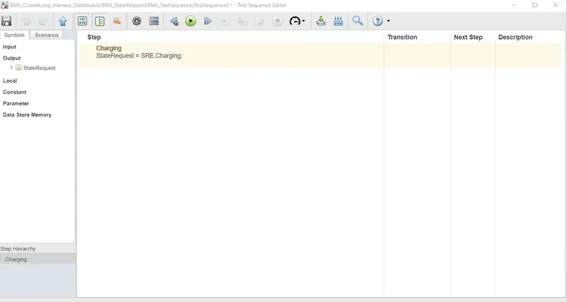
State Request Data -

Results -

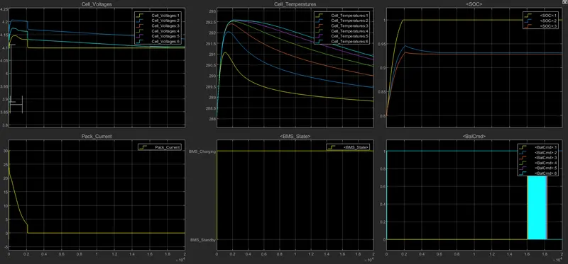
Cell Voltage and Pack Current -

• Cell 1 voltage rise from 3.85V to 4.1V and become constant at 4.08V.
• Cell 2 voltage increases from 3.9 to 4.2 V and Stabilizes at 4.15 V.
• The pack current is increased to 30A and is stabilized at 3A. After 2000 Sec the battery is fully charged and the current is dropped to 0A.

Temperature -

• The temperature of the cells is increased abruptly during charging and is reduced gradually once the charging is complete and the temperature stabilizes at ambient temperature.
• The maximum temperature is achieved by cell 6 at 292.5K which is lower then the discharge temperature.

BMS Status -

• The entire BMS is operating at Charging Phase.

SOC -

• The SOC is charged at 93% According to UKF and EKF method while according to the Columb Counting method the battery is 100 percent charged.

Balancing Command -

• Cell 6 and cell 2 are balanced from the start while the rest of the cells are balanced at the end of the simulation.

(B) Understanding SOC using coulomb counting method.

State of Charge or SOC can be defined as the charge available in a battery at any instant of time. The SOC is an estimate of the remaining energy capacity of the battery as compared to its fully charged rate.

In the Coulomb Counting Method, we integrate the charging current over the period of discharge and Calculate the SOC against the 100% Capacity value.

`SOC(t)=SOC(t-1)+((I(t))/Q_n*t)`

SOC model -

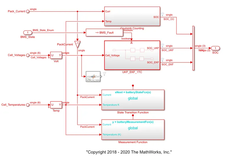
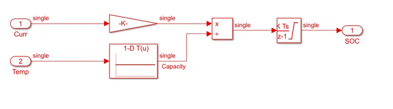
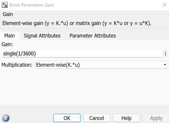
• The Subsystem uses current as input and a Gain block is used to convert the current into Ah values by using a Gain block.
• A 1-D look-up table is used to define the Maximum capacity at different temperatures.
• A discreet time integrator block is used to integrate the Current values with real-time.

The Above block Diagram is used to Simulate the Coulomb counting method in the BMS ECU project.