Aim:-
Simulation of a 1D supersonic nozzle flow simulation using
in this challenge you are going to simulation the isortopic flow through a 1D subsonic-supersonic nozzle .
you will derive both the conservation and non -conservation forms of the governingquatiorand solve them using the macrocosm's technique.
you need to determine the steady-state temperature distribution for the flow -field variable and investigate the difference between the two forms of governing quotations by comparing this solutions.
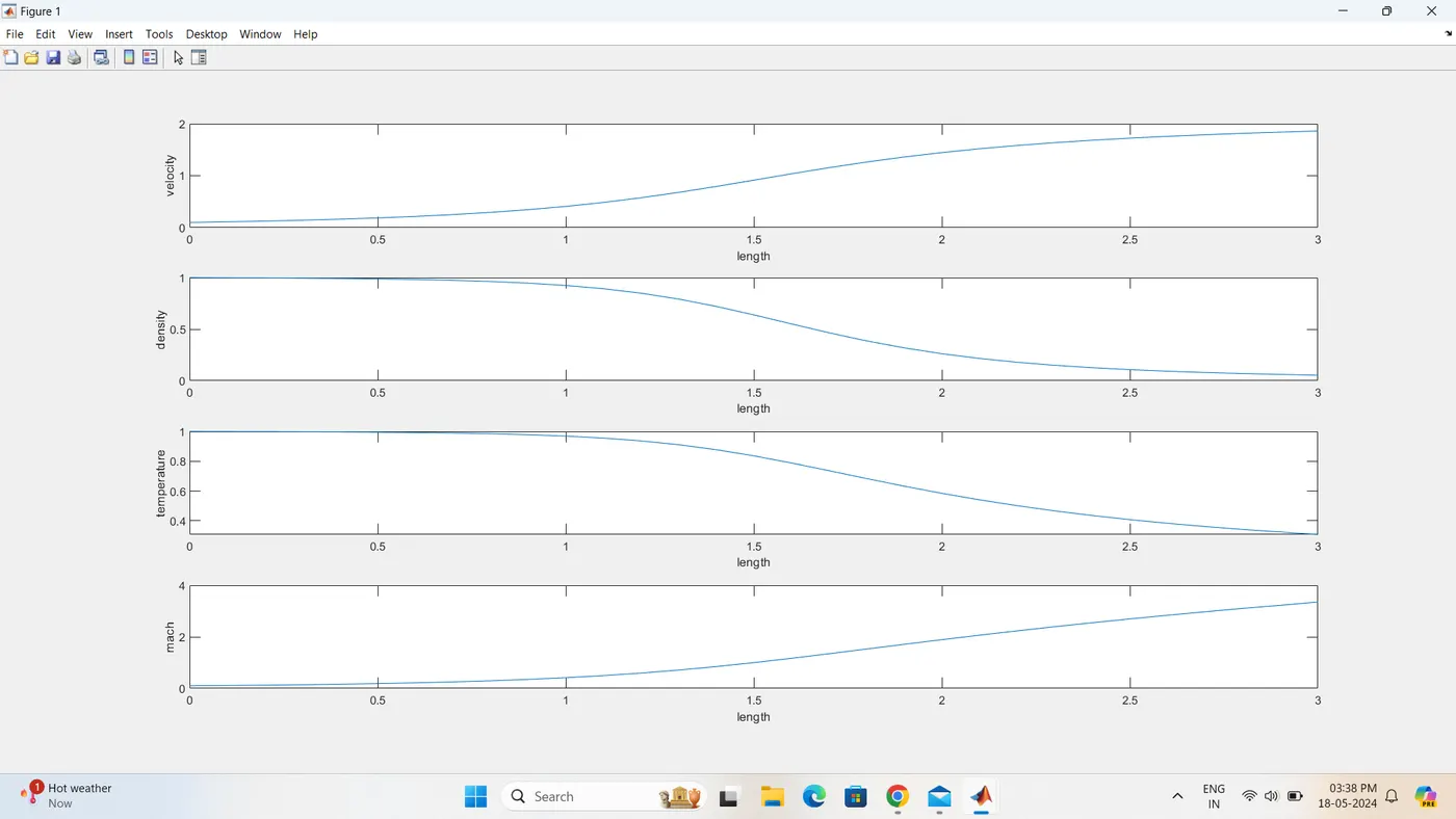
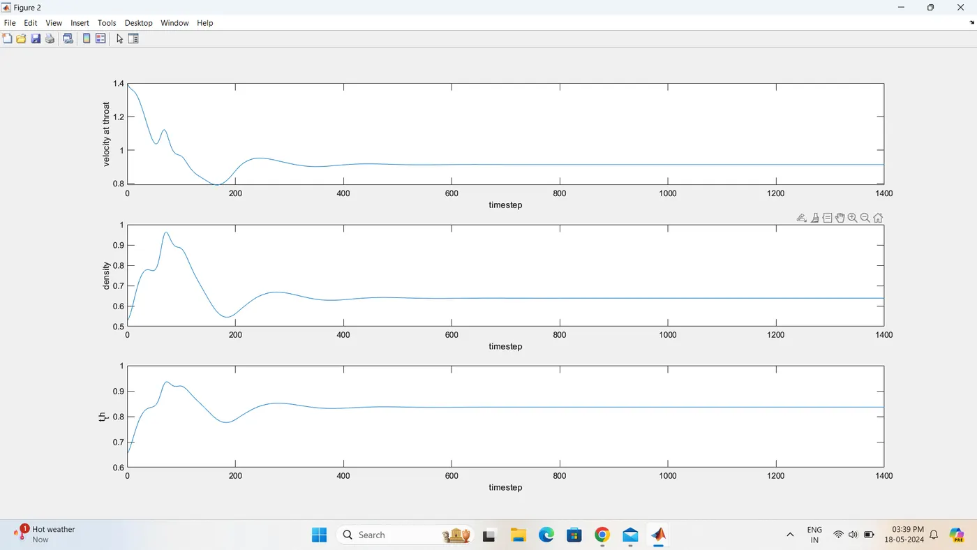
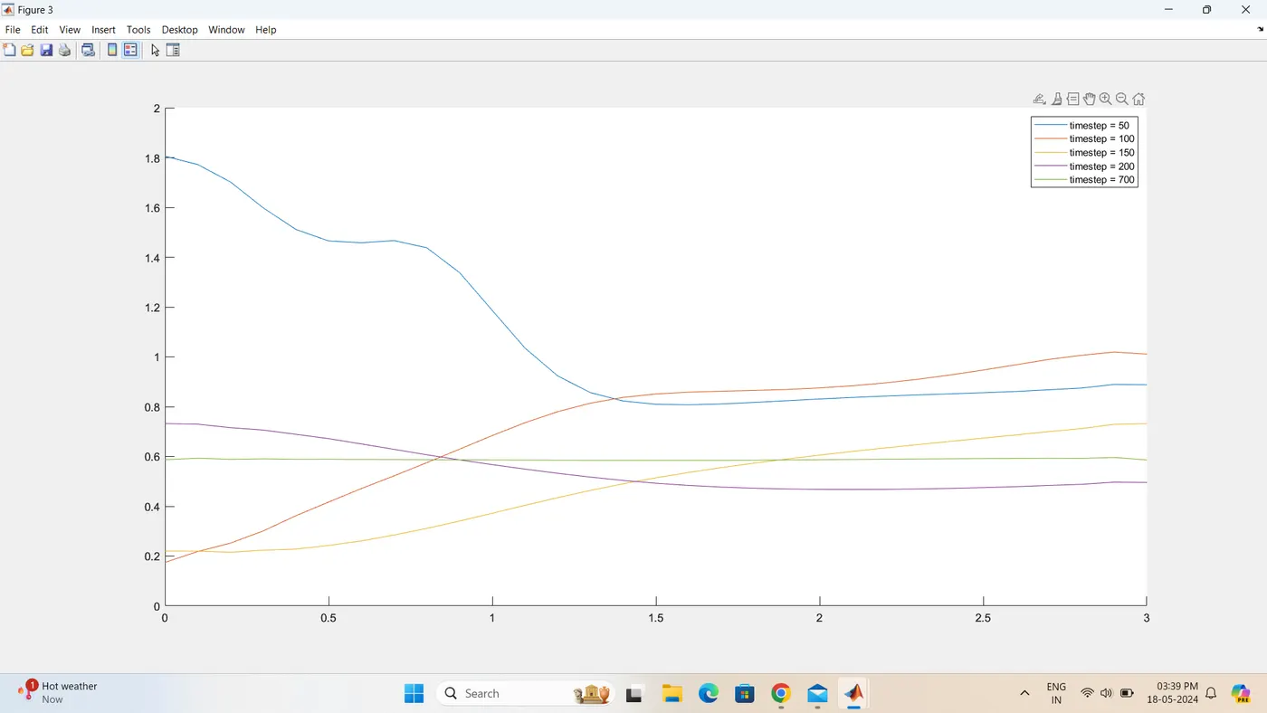
you need to show the following plots inside your report
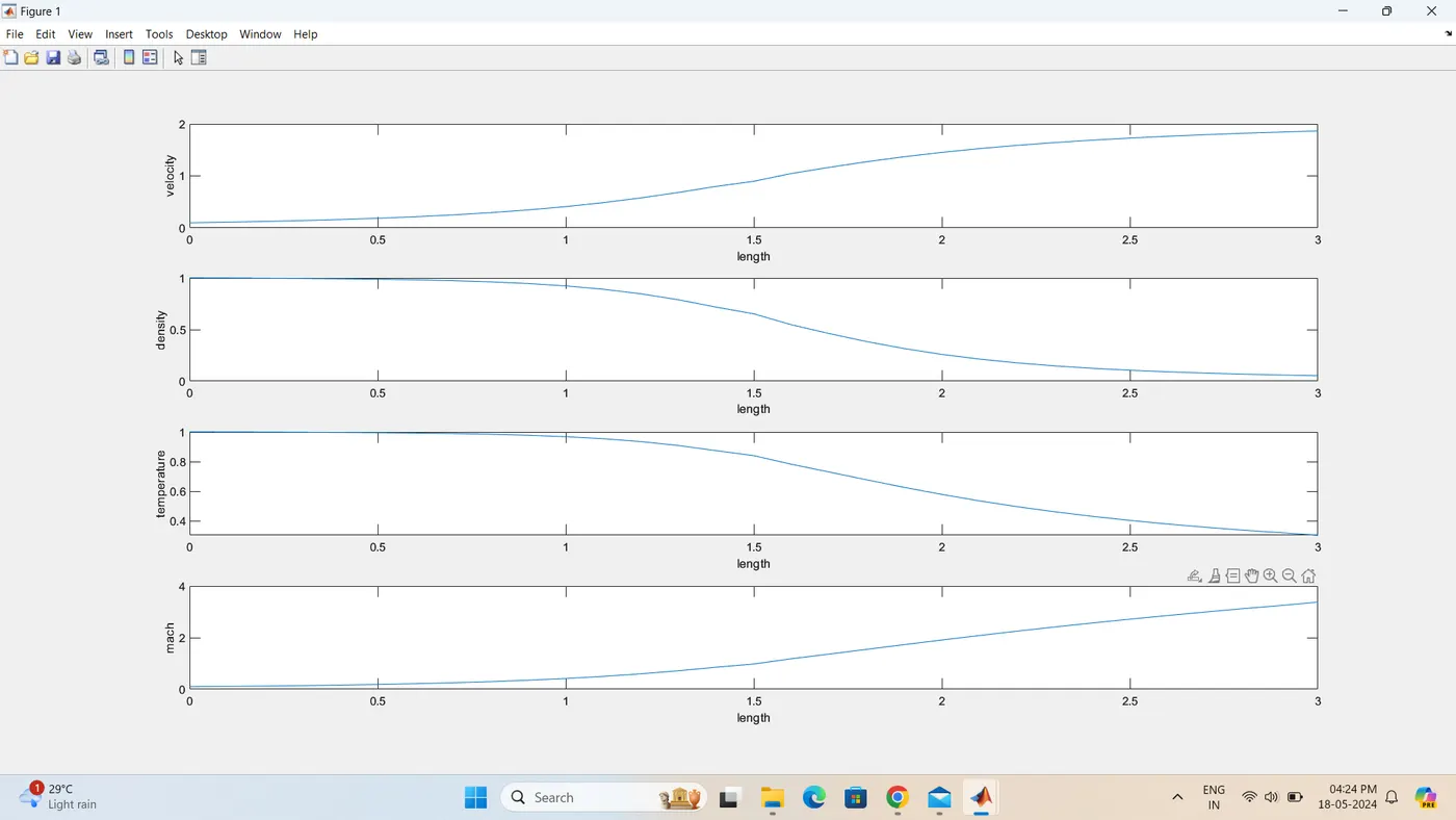
1.Steady-State distribution of primitive variablrs inside the nozzle
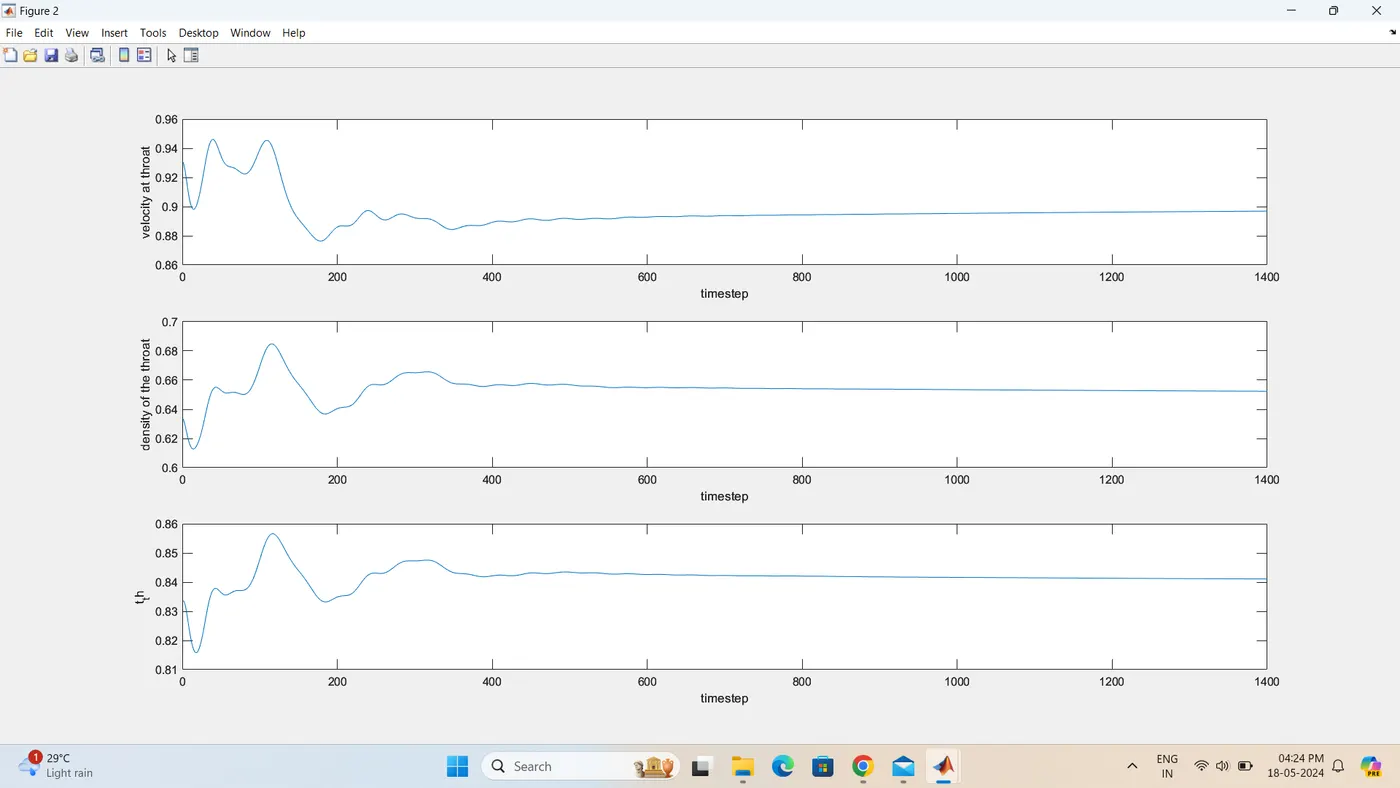
2.Time -wise variation of the primitive variables
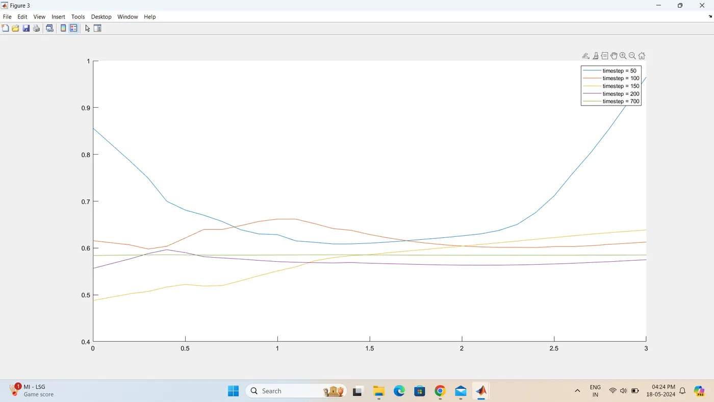
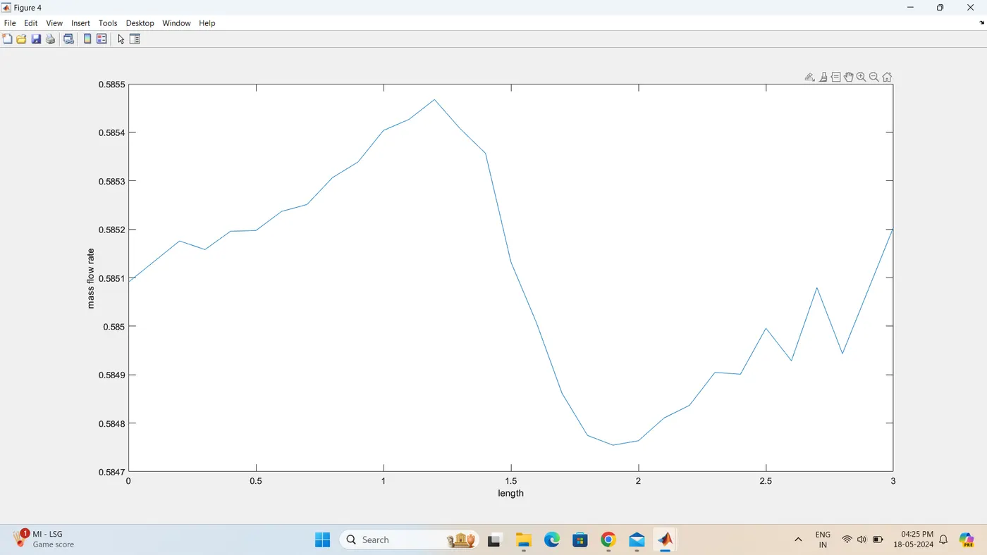
3.Variation of mass flow rate disteibution inside the nozzle at different tome steps during the time-marching process
4.Comparison if Normalized flow through the convergent nozzle as give in diagram below
INTRODUCTION TO THE GIVEN PROBLEM
We consider the steady isntropic flow theougth the convergent -divergent as given in diagram below .
We consider the steady isontropic flow throughr the convergent -divergent nozzle aas given in diagram below
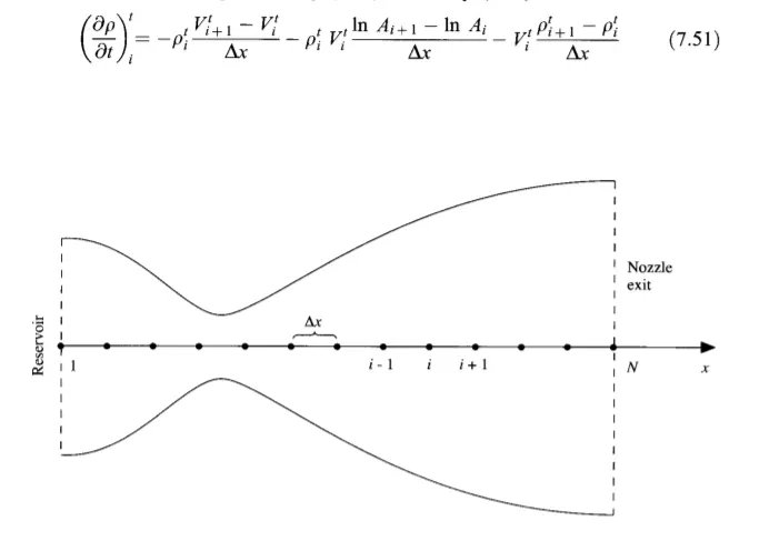
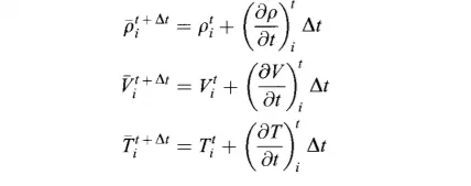
Momentum equation
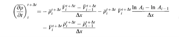

Energy equation
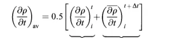
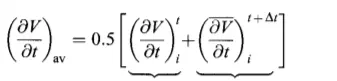
Calculation of Average
its basically the half of the sum of corrector and predictor value.
2)
3)

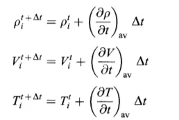
Density and Temperature at point 1 is held fixed.

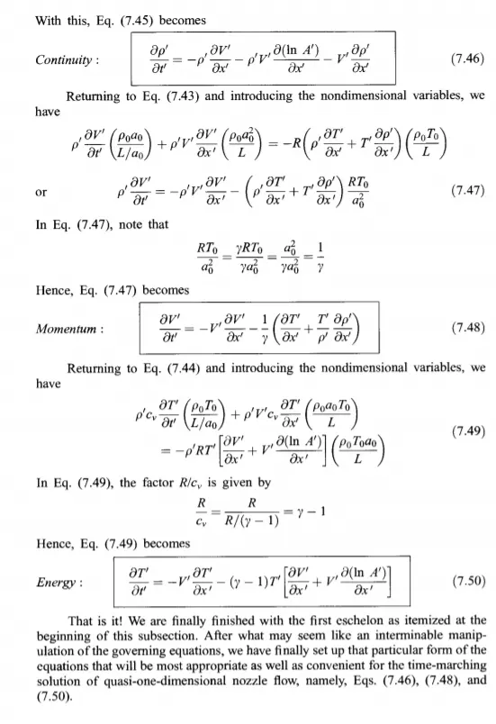
The momentum equation
The energy equation :

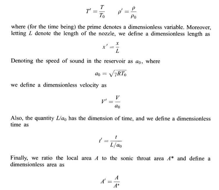
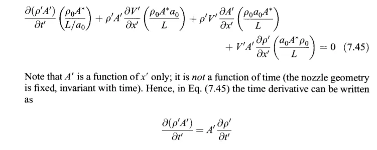
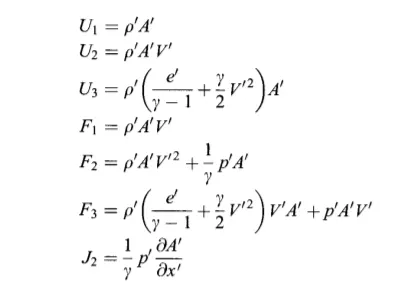
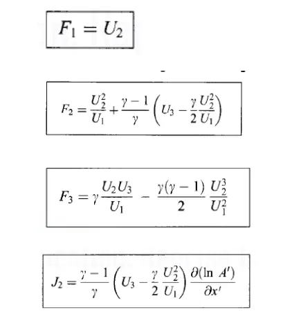
The above are the non dimansional conservation form of the coninutiy ,Momentum and energy equation The quasi-one -dimansinal floe ,respectiveley.The equations for quasi one dimensional flow can be expressed in generic form. Let us define the elements of the solution vector U, flux vector F and the source term J as follows
From the above equations we can write that
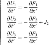
These are the equations we wish to solve numerically by using the MacCormacks technique.
To obtain the primitve variables we must decode the elements U1,U2,U3 as follows.From the defination of U1,U2 and U3 given above we have
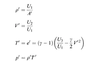
Expressing the flux and source term in form of solution vectors
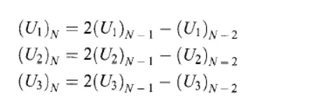
Applying the boundry conditions:
Initial conditi
%inputs
n=31;
x = linspace(0,3,n);
dx = x(2)-x(1);
%calculate the initial profiles
rho = 1-0.3146*x;
t = 1-0.2314*x;
v =(0.1+1.09*x).*t.^0.5;
gamma = 1.4:
%calculate the are
a = 1+2.2*(x-1.5).^2;
pos = find(a==min(a))
%time step
nt = 1400;
cfl=0.5;
dt = min (cfl.*dx/sqrt(t)+v));
%outer time loop
for k = 1:nt
%preditor method
rho_old=rho;
v_old=v;
t-old=t;
for j = 2:n-1
dvdx = (v(j+1)-v(j))/dx;
drhodx = (rho(j+1)-rho(j))/dx;
dtdx=(t(j+1)-t(j))/dx;
dlogadx=(log(a(j+1))-log(a(j)))/dx;
%continuty equation
drhdt_p(j) =-rho(j)*dvdx-rho(j)*(j(*dlogadx-v(j)*drhodx;
%momentum equation
dvdt_p(j)*dvdx-(1-gamma)*(ddtdx+(t(j)/rho(j)*drhodx);
%energy ewuation
dtdt_p(j)= -v(j)*dtdx-(gamma-1)*t(j)*(dvdx+v(j)*dlogadx);
%solution update
v(j)=v(j)+dvdt_p(j)*dt;
rho(j)=rho(j)-drhodt_p(j)*dt;
t(j)=t(j)+dtdt_p(j)*dt;
end
%corrector method
for j =2:n-1
dvdx =(v(j)-v(j-1))/dx;
drhodx=(rho(j)-rho(j-1))/dx;
dtdx=(t(j-1))/dx;
dlogadx=(log(a(j))-loga(j-1)))/dx;
%continuty equation
drhodt_c(j)=-rho(j)*dvdx-rho(j)*cv(j)*drhodx;
%momentum equation
dvdt_c(j) =-vdvdx-(1/gamma)*(dtdx+(t(j)/(j))*drhodx);
%energy equation
dtdt_c(j)=-v(j)*dtdx-(gamma-1)*t(j)*(dvdx+v(j)*dlogadx);
end
%computer the avrage time derivative
drhodt =0.5*(drhodt_p+drhodt_c);
dvdt=0.5*(dvdt_p+dvdt_c);
dtdt=0.5*(dtdt_pdtdt_c);
%final solution update
foe i = 2:n-1
rho(i) =rho_old(i)+drhodt(i)*dt;
v(i)= v_old(i)*dt;
t(i)=t+old(i)+dtdt(i)*dt;
end
%apply the boundary conditions
%inlet
v(1)=2*v(2)-v(3);
rho(n)=2*rho(n-1)-t(n-2);
rho_th(k)=rho(pos);
t_th(k)=t(pos);
v_th(k)=v(pos);
mdot=rho.*a.*v;
fihure(3)
hold on
if k==50
pilt(x,mdot)
end
if k==100
plot(x,mdot)
end.if k==200
plot(x,mdot)
end
if k==150
plot(x,mdot)
end
if k==200
plot(x,mdot'display',dfasdfa')
end
end
legend('timestep=50','timestep=100','timestep=1500','timestep=200','timestep=700')
mach=v./sqrt(t)
figure(1)
subplot(4,1,1)
plot(x,v)
xlabel('lenght')
subplot(4,1,1)
plot(x,v)
xlabel('lenght')
ylable('density')
subplot(4,1,3)
plot(x,t)
xlabel('lendht')
ylabel('temperate')
subplot(4,1,4)
plot(x,mach)
figure(2)
subplot(3,1,)
plot(v_th)
xlabel('timestep')
ylabel('velocity at throat')
ylabel('velocity at throat')
subplot(3,1,2)
plot(rho_th)
xlabel('timestep')
ylabel('density')
sunplot(3,1,3)
plot(t_th)
xlabel('timestep')
ylabel('t_th')
figure(4)
plot(x,mdot')
xlabel('lenght')
ylabel('mdot')
os =
plot(x,mdot)
xlabel('length')
pos =
16
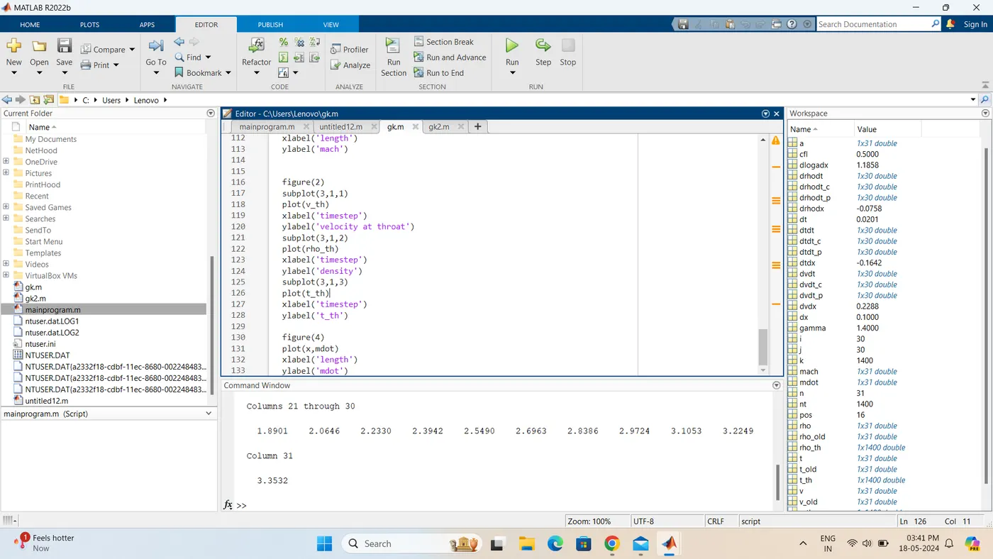
mach = cloumns 1 through 10
0.0988 0.1121 0.1253 0.1428 0.1625 0.1870 0.2162 0.2521 0.2958 0.3496
columns 11 through 20
0.4155 0.4962 0.5938 0.7103 0.8459 0.9994 1.1674 1.3451 1.5276 1.7103
columns 21 through 30
1.8901 2.0646 2.2330 2.3942 2.5490 2.6963 2.8386 2.9727 3.1053 3.2249
column 31
3.3532
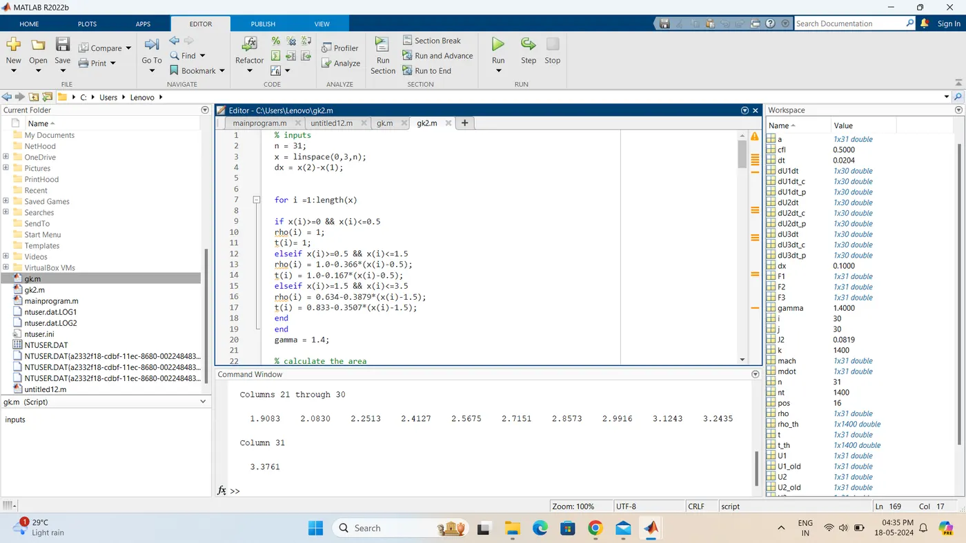
Matlab program non -conservation
n =31;
x= linspace(0,3,n);
dx = x(2)-x(1);
for i =1:length(x)
if x(i)=1;
rho(i)= 1;
t(i)=1;
elseif x(i)=1.5&&x(i)<=0.5
rho(i)=1.0-0366*(x(i)-0.5);
t(i)=1;
elself x(i)>=0.5&&x(i)-0.5)
rho(i) =1.0-0.366*(x(i)>-0.5);
t(i) = 1.0-0.167*(x(i)-0.5);
elseif x(i)>=1.5&&x(i)-1.5);
t(i)= 0.833-0.3507*(x(i)-1.5);
end
end
gamma =1.4;
%co=alculate the area
a = 1+2.2*(x-1.5).^2;
pos = find(a==min(a))
v = 0.59./(rho.*a);
% time steps
nt = 1400;
clf = 0.5;
dt =min(clf.*dx./(sqre(t)+v));
% declaarang U1 U2 and U3
U1 =rho.*a;
U2 = rho.*a.*v;
U3 = rho.*a.*((t/gamma-1))+(0.5*gamma.*v.^2));
for k = 1:nt
% predictior method
U1_old =U1;
U2-old = U2;
U3_old = U3;
F1 =U2;
F2 = (U2.^2./U1)+(gamma-1)).*(U3-0.5*gamma*(U2.^2./U1));
F3 =(gamma*U2.*U3./U1)-(0.5*(gamma^2-gamma)*(U2.^3./U1.^U1.^2));
for j = 2:n-1
J2 = (1/gamma).*rho(j).*(j).*(-a(j+1)-a(j))/dx;
%continuty equation
dU1dt-p(j) = -F1(j+1)-f1(j))/dx;
%momentum equation
dU2dt-p(j) =-F2(j+1)-F1(j))/dx+j2;
%energy equation
dU2dt-p(j) =-(f3(j+1)-F3(j))/dx;
%solution update
U1(j) = U1(j)+dU1dt-p(j)*dt;
U2(j) = U2(j)+dU2dt-p(j)*dt;
U3(j) = U3(j)+dU3dt-p(j)*dt;
end
%update of varibles
rho = U1./a;
t = (gamma-1).*((U3./U1)-((0.5*gamma)*(U2./U1).^2));
v = U2./U1;
%update the flux vector
F1 = U2;
F2 =(U2.^2./U1) +(gamma^-1*(gamma-1)).*(U3-0.5*gamma*(U2.^2./U1));
F3 = (gamma*U2.*U3./U1)-0.5*(gamma)*(U2.^3./U1^^2));
%correction methode
for j= 2:n-1
J2 = (1/gama).*rho(j).*t(j).*(a(j)-a(j-1))dx;
%continuty equation
dU1dt_c(j0= -(f1(j)-f1(j-1))/dx;
%momentum equation
dU2dt_c(j)=-(f2(j)-f2(j-1))/dx+j2;
%energy equation
dU3dt_c(j)=-f3(j)-f3(j-1))/dx;
end
%Computer the average time derivative
dU1dt =0.5*(dU1dt_p+dU1dt_c) ;
dU1dt =0.5*(dU1dt-P+dU1dt_c);
d2Udt =0.5*(dU1dt_p+dU2dt_c);
dU3dt = 0.5*(dU3d_p+dU3dt_c);
% final solution update
for i= 2:n-1
U1(i) = U1_old(i)+dUdt(i)*dt;
U2(i) = U2_old(i)+dU2(i)*dt;
U3(i) = U3_old(i)+dU3dt(i)*dt;
end
%apply the boundary conditions %inlet
U1(1)= rho(1).*a(1);
Y2(1) =2*U2(2)(3);
U3rho(1).*a(1).*((t(1)/(gamma-1))+ (0.5*gamma.*v(1).^2));
%outlet
U1(n)=2*U1(n-1)-U1(n-2);
u2(n) =2*U2(n-1)-U2(n-2);
U3(n)=2*U3(n-1)-U3(n-2);
%calculating the primatives
rho= U1./a;
v=U2./U1;
t=(gamma-1).*((U3./U1)-((0.5*gamma)*(U2./U1).^2));
rho_th(k) =rho(pos);
t_th(k)= t(pos);
v_th(k) =v(ops);
mdot = rho.*a.*v;
figure(3)\
hold on
if k==50
plot(x,mdot)
end
if k==100
por(x,mdot)
end
if k ==150
plot(x,mdot)
end
if k==200
plot(x,mdot)
end.if k==700
plot(x,mdot,'display',dfasdfa')
end
end
legend('timestep =50',timeset =100',timeset=150',timestep=200',timestep=700')
mach=v./sqrt(t)
figure(1)
subplot(4,1,1)
plot(x;v)
xlabel('lenght')
ylabel('velocity')
subplot(4,1,2)
plot(x,rho)
xlable('length')
ylable('density')
subplot(4,1,3)
plot(x,t)
xlabel('lenght')
ylable('temperature')
subplot(4,1,4)
plot(x,mach)
xlabel('lenght')
ylanel('mach')
figure(2)
subplot(3,1,1)
plot(v_th)
xlable(timeatep')
ylable('velocity at throst')
subplot(3,1,2)
xlabel(rho_th)
ylable('density of the throat')
subplot(3,1,3)
plot(t_th)
xlabel('timestep')
ylabel(t_th')
figure(4)
plot(x,mdot)
xlabel('lenght')
ylabel('mass flow rate')
pos=
16
mach =
columns 1 through 10
0.0983 0.1103 0.1245 0.1413 0.1614 0.1856 0.2150 0.2500 0.2949
columns 11 through 20
0.4158 0.4976 0.5970 0.7155 0.8535 0.9780 1.1826 1.3616 1.5451
1.7383
columns 21 thought 30
1.9083 2.0830 2.2513 2.4127 2.5675 2.7151 2.8573 2.9916 3.1243 3.2435
column
31 3.3761