Challenge

Week 7 - Simulation of a 1D Supersonic nozzle flow simulation using Macormack Method

CChinmay Jangale12 Sept 2023

Question:

In this challenge you are going to simulate the isentropic flow through a quasi 1D subsonic-supersonic nozzle. You will derive both the conservation and non-conservation forms of the governing equations and solve them using the MacCormack's technique. You need to determine the steady-state temperature distribution for the flow-field variables and investigate the difference between the two forms of governing equations by comparing their solutions.

Objectives:

You need to show the following plots inside your report
1. Steady-state distribution of primitive variables inside the nozzle
2. Time-wise variation of the primitive variables
3. Variation of Mass flow rate distribution inside the nozzle at different time steps during the time-marching process
4. Comparison of Normalized mass flow rate distributions of both forms

Solution:

Here we goanna solve the Quasi 1D subsonic-supersonic nozzle in two different forms conservative form and non-conservative form;

Governing equations:

· Conservative equation and one conservative form of equation are mathematically equivalent.

· One com can be converted into another form. Quite easily and exactly.

· Conservative and non-conservative are different only in world of numerical discretization.

· Whereas conservative form are more accurate and it tends to work well Discontinuities, Exist in domain

Whereas our domain looks like the figure given below, in which we say it as 1D flow but in actual it is 2D only. During inlet and divergent the Mach number is Going to be less than one. Whereas at subsonic calculate the Mac number will be larger than one. So in this challenge we are going to see. Behavior of the Mach number of pressure temperature and density throughout the nozzle.

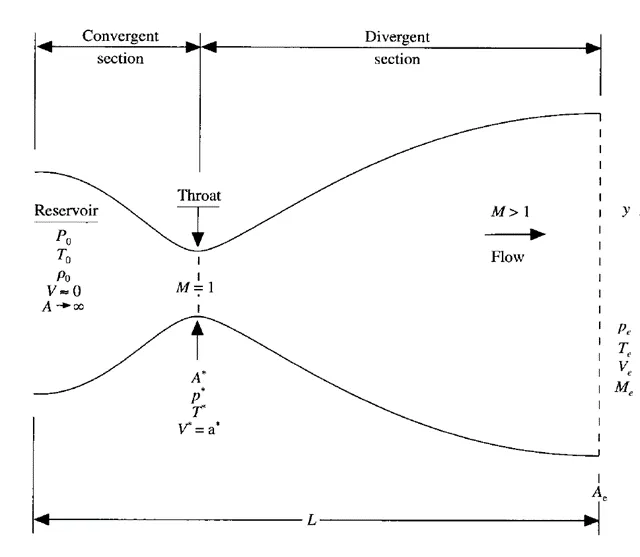
Fig 1. 1D subsonic-supersonic Nozzle

Now lets derivative first non-conservative form and then conservative form mathematically;

1.NON-CONSERVATIVE FORM:

We have Rate of change of mass;

`∫∫∫(∂/(∂t))(ρ dv)=∂/(∂t)∫∫∫ρ.dv`

Where `(ρ.dv)` is control volume and above equation is also equal to “inflow – outflow ” and equalize to negative of surface integral.

“The only mass entering of exiting will be through one of the triangle which is going to be surface integral”

Surface integral is `=-∫∫ρ.v.ds` ;

So, the equation now becomes;

`∂/(∂t)∫∫∫ρ.dv+∫∫ρ v ds=0` ……………………1

Where ds is control volume which we can see in fig.2 , in which we put the slice of nozzle flow, where the thickness of slice is dx. Where on left side control volume consistent. With quasi 1D assumption. The density velocity pressure and integral energy is noted by ρ V P and E. respectively are uniform over the area a similarly right side of the control volume. The density velocity pressure and integral energy denoted by ρ+dρ, v+dv, p+dp and e+de respectively are uniform over the area A+dA.

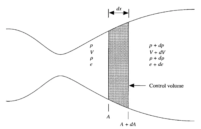
Fig 2. Control volume

Therefore;

`∂/(∂t)∫∫∫ρ dv=∂/(∂t)∫∫∫ρ A dx=∂/(∂t) (ρA)dx`

Surface integral term will be,

`∫∫ρ v ds=-ρvA+(ρ+dρ)(v+dv)(A+dA)`

After simplifying above term and ignoring all small terms for example multiplication of dA, dv and dρ. Because as dx is small All these differences are small and product of these differences are even more small.

Term remains will be;

`∫∫ρ v ds=ρAdv+dρAv+ρvdA`

If we see above term, we can see it is application of chain rule (simplification of above term),

`∫∫ρ v ds=d(ρAv)`………………….2

If we put equation 2 in equation 1 we get;

`∂/(∂t) (ρAdx)+d(ρAv)=0` …………………3

Dividing equation 3 by dx, we get

`∂/(∂t) (ρA)+∂/(∂x) (ρAv)=0` …………….4.1

Equation 4 is the partial differential equation form of continuity equation suitable for unsteady passive 1 dimensional flow. It ensures that mass is conserved for this model of flow It is interesting to pause at a moment and compare this with a general continuity equation. Part 3D flow specialise for one day if flow for such case equation becomes

`(∂ρ)/(∂t)+(∂(ρv))/(∂x)=0`

Where V is X component of velocity, clearly equation is different from equation 4 above equation applies to truly 1D flow, where A is constant with respect to X. It does not represent proper statement of conservation of mass for our model of Quasi 1D flow, where A is equal to A(x) Instead, equation 4 is proper statement of mass conservation for our model. Of course, note that for the special case of constant area flow, equation 4 Reduce to above equation.

Now from above continuity equation we get the momentum equation as it is long derivation part and we don’t need to involve in that so we write here directly;

`∂/(∂t) (ρAv)+∂/(∂x) (ρAv^2 )=-A (∂p)/(∂x)` ………….4.2

Above term represents the momentum equation and both the term continuity and momentum are in conservative form and to make it in non-conservative form we need to apply the u*v rule using that rule we get the non-conservative form of continuity and momentum equation;

`∂/(∂t) (ρA)+v ∂(ρA)/(∂x)=-ρA (∂v)/(∂x)` …………. continuity equation in non-conservative form

`ρ (∂v)/(∂t)+ρv (∂v)/(∂x)=-(∂p)/(∂x)` ………………. Momentum equation in non-conservative form

Energy equation will be;

`∂/(∂t) (ρ v^2/2 A)+∂/(∂x) (ρ v^3/2 A)=-Av (∂ρ)/(∂x)` ………..4.3

In non-conservative form;

`ρ(∂T)/(∂t)+ρv(∂T)/(∂x)=-p(∂v)/(∂x)-pv(∂(lnA))/(∂x)` ……………Energy equation in non-conservative form

As an incident, somebody our continuity momentum and energy equation for unsteady quasi red one dimensional flow are given by above equations. See, you see three equation with the unknown variables. Rho V, P and T. The pressure can be eliminated from this equation by using the equation of state.

`p=ρRT`

Along with its derivative;

`(∂ρ)/(∂x)=R(ρ (∂t)/(∂x)+T (∂ρ)/(∂x))`

With this the governing equations will be;

`∂/(∂t) (ρA)+ρv (∂(A))/(∂x)+ρA (∂v)/(∂x)+vA (∂ρ)/(∂x)=0` ………. Continuity equation

`ρ (∂v)/(∂t)+ρv (∂v)/(∂x)=-R(ρ(∂T)/(∂x)+T (∂p)/(∂x))` ………. Momentum equation

`ρ (∂T)/(∂t)+ρvc_v (∂T)/(∂x)=-ρRT[(∂v)/(∂x)+v (∂(lnA))/(∂x)]` …. Energy equation

At this stage, we could really proceed to set up an readily solution of above continuity momentum and energy equation. Note that these are written in terms of dimension variable. This is fine and many CFD solution are carried out directly in terms of such, dimensional variable. Indeed, this has an added engineering advantage, because it gives you feeling for the magnitude of real physical quantities as the solution progresses. However, for nozzle flows the flow field variable are frequently expresses in terms of non-dimensional variable. Where the flow variable p/p0, ρ/ρ0, and T/T0 vary between 0 and 1 which is an aesthetic advantage when presenting the result. Because fluid dynamics dealing with nozzle flow so frequently use this non-dimensional term.

Therefore, where the Reservoir temperature and density are denoted by T0 and ρ0 respectively. Define the non-dimensional temperature and density respectively as;

`T^'=T/T_0 ; ρ^'=ρ/ρ_0 ;`

Where the prime denotes a dimensionless variable moreover letting l denote the length of nozzle we define a dimensional less length as;

`x^'=x/L`

Denoting the speed of sound in reservoir as a₀ where;

`a_0=√γRT_0`

We define dimensionless velocity as ;

`v^'=v/a_0`

Finally, we ratio the local area A to the sonic throat area A* and define a dimensionless area as;

`A^'=A/(A^*)`

Now as we have set of governing equations, variables now let’s see the methodology;

`(∂(ρ^' A^' ))/(∂t) ((ρ_0 A)/(L/a_0 ))+(ρ^' A^' ∂v^')/(∂x^' ) ((ρ_0 Aa_0)/L)+(ρ^' v^' ∂A^')/(∂x^' ) ((ρ_0 Aa_0)/L)+(v^' A^' ∂ρ^')/(∂x^' ) ((ρ_0 Aa_0)/L)`

Note that A is function of x only; it is not a function of time hence in above equation the time derivative can be written as ;

`(∂(ρ^' A^' ))/(∂t^' )=A^' (∂ρ')/(∂t')`

The continuity equation becomes;

`(∂ρ^')/(∂t^' )=-ρ^' (∂v^')/(∂x^' )-ρ^' v^' (∂(lnA^' ))/(∂x^' )-v^' (∂ρ^')/(∂x^' )` ………….C

And similarly we get another equations

Momentum equation becomes

`(∂v^')/(∂t)= -v (∂v^')/(∂x^' )-(1/γ)((∂T^')/(∂x^' )+T^'/ρ^' ((∂ρ^')/(∂x))` …………..M

Energy equation becomes;

`(∂T^')/(∂t^' )=-v^' (∂T^')/(∂x^' )-(γ-1) T^' [(∂v^')/(∂x^' )+v^' (∂(lnA^' ))/(∂x^' )]` ……. E

Methodology:

1. Mesh

2. Discretize

3. Solve conditions

· Initial condition

· Boundary condition

Where in one dimensional domain the mesh looks like breaking of line in different parts or dividing that line by number of nodes we want.

But discretization we are going to do is using MacCormack technique;

1.1.MacCormack technique

McCormack technique is variant of lax Wendorff approach. But is much simpler in its application. McCormack is also an explicit finite difference technique, which is second order accurate in both space and time It becomes most popular, explicit, finite difference method for solving fluid flow.

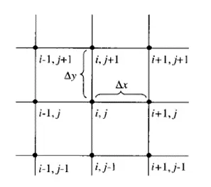
Fig 3. 2D Grid

In above fig there is two-dimensional grid where we will address time marching solution using MacCormack technique as before we assume flow field at each grid point is known as time(t) and we proceed to calculate flow field variables at same grid point at time t+∆t.

First consider the density at grid point (i,j) at time (t+∆t), in McCormack method this is obtain from;

`ρ_(i,j)^(t+∆t)=ρ_(i,j)^t+((∂ρ)/(∂t))_(avg) ∆t` …………….5

Where drho/dt represents mean value of drho/dt between times t and t+∆

The time derivative are equivalent at time and carrying out second derivative. Is necessary to obtain 2^nd order accuracy In contrast equation 5 the value of dp/dt is calculated.

So as to preserve second order accuracy without the need of calculate value of 2^nd time derivative which is term in which involves lot of algebra with McCormack technique This algebra is circumvented.

Similar relation are written for other flow field variables

`u_(i,j)^(t+∆t)=u_(i,j)^t+((∂u)/(∂t))_(avg) ∆t` ………………6

`v_(i,j)^(t+∆t)=v_(i,j)^t+((∂v)/(∂t))_(avg) ∆t` ………………7

`e_(i,j)^(t+∆t)=e_(i,j)^t+((∂e)/(∂t))_(avg) ∆t` ……………….8

Now let’s see how we calculate the average value of derivative;

There are two major steps in McCormack technique which is predictor and corrector step,

1.1.1.Predictor step

In continuity equation 5 replace the spatial derivative on right hand side with forward differences.

`((∂ρ)/(∂t))_(i,j)^t=-[ρ_(i,j)^t (u_(i+1,j)^t-u_(i,j)^t)/∆x+u_(i,j)^t ((ρ_(i+1,j)^t-ρ_(i,j)^t ))/∆x+ρ_(i,j)^t ((v_(i,j+1)^t-v_(i,j)^t)/∆x)+v_(i,j)^t ((ρ_(i,j+1)^t-ρ_(i,j)^t)/∆x)]` …………9

In equation 9 all flow variable at Time (t) are nonvalues. That is, right hand side is known. Now obtain predicted value of density for first two term of Taylor series as follow;

`ρ_(i,j)^(t+∆t)=ρ_(i,j)^t+((∂ρ)/(∂t))_(i,j)^t ∆t` …………...10

In equation 10 ρ_i,j^t is known and (dρ/dt)^t_i,j . Is known from equation 9  is only predictable value of density. It is only first order accurate since equation 10 contains only first order term in Taylor series.

And similarly for other variables;

`u_(i,j)^(t+∆t)=u_(i,j)^t+((∂u)/(∂t))_(i,j)^t ∆t`……………11

`v_(i,j)^(t+∆t)=v_(i,j)^t+((∂v)/(∂t))_(i,j)^t ∆t` …………….12

`e_(i,j)^(t+∆t)=e_(i,j)^t+((∂e)/(∂t))_(i,j)^t ∆t` …………….13

1.1.2. Corrector step

In character state, we first obtain a predictor value of time derivative at time t+∆t, `((∂ρ)/(∂t))_(i,j)^(t+∆t)`By substituting the predicted value of rho, u and v into right side of continuity equation, replacing spatial derivatives with backward differencing.

`((∂ρ)/(∂t))_(i,j)^(t+∆t)=-[ρ_(i,j)^(t+∆t) (u_(i,j)^(t+∆t)-u_(i-1,j)^(t+∆t))/∆x+u_(i,j)^(t+∆t) ((ρ_(i,j)^(t+∆t)-ρ_(i-1,j)^(t+∆t) ))/∆x+ρ_(i,j)^(t+∆t) ((v_(i,j)^(t+∆t)-v_(i,j-1)^(t+∆t))/∆x)+v_(i,j)^(t+∆t) ((ρ_(i,j)^(t+∆t)-ρ_(i,j-1)^(t+∆t))/∆x)]` …14

The average value of time derivative of density, which appears in equations 5 is obtained from arithmetic mean of. `((∂ρ)/(∂t))_(i,j)^t` obtain from equation 9 and `((∂ρ)/(∂t))_(i,j)^(t+∆t)`from equation 14.

`((∂ρ)/(∂t))_avg=0.5[((∂ρ)/(∂t))_(i,j)^t+((∂ρ)/(∂t))_(i,j)^(t+∆t) ]` …………..15

Equation 15 allow us to obtain final corrected value of density at time (t+∆t) from equation 5. Repeated below

`ρ_(i,j)^(t+∆t)=ρ_(i,j)^t+((∂ρ)/(∂t))_(avg) ∆t`

The Mccomack technique as described above because two step predictor and corrector sequence is used with forward differences on predictor and backward differences on corrector is second order accurate method.

Coming back to non-conservative form;

Using the McCormack technique our governing equation for predictor step we get is (with ref to equation 9);

From continuity equation;

`((∂ρ)/(∂t))_(i,j)^t=-[ρ_(i,j)^t ((v_(i+1)^t-v_i^t)/∆x)+ρ_i^t v_i^t ((ln⁡〖A_(i+1)-lnA_i 〗 ))/∆x+v_(i,j)^t ((ρ_(i+1)^t-ρ_i^t)/∆x)]`……16

From momentum equation;

`(∂v^')/(∂t)= -v((v_(i+1)^t-v_i^t)/∆x)-(1/γ)(((T_(i+1)^t-T_i^t)/∆x)+T^'/ρ^' ((ρ_(i+1)^t-ρ_(i,)^t)/∆x))` ……………17

From energy equation:

`(∂T^')/(∂t^' )=-v^' ((T_(i+1,j)^t-T_(i,j)^t)/(∆x))-(γ-1) T^' [((v_(i+1,j)^t-v_(i,j)^t)/(∆x))+v^' ((ln⁡〖A_(i+1)-lnA_i 〗 ))/(∆x)]` ………18

Using equation 10 we know;

`ρ_(i,j)^(t+∆t)=ρ_(i,j)^t+((∂ρ)/(∂t))_(i,j)^t ∆t` ………..19.a

`v_(i,j)^(t+∆t)=v_(i,j)^t+((∂v)/(∂t))_(i,j)^t ∆t` ………..19.b

`T_(i,j)^(t+∆t)=T_(i,j)^t+((∂T)/(∂t))_(i,j)^t ∆t` ………..19.c

Moving to corrector step, we return to our governing equations and apply the spatial derivative with backward differencing this time;

`((∂ρ)/(∂t))_(i,j)^(t+∆t)=-[ρ_(i,j)^t ((v_(i,)^t-v_(i,-1)^t)/(∆x))+ρ_i^t v_i^t ((ln⁡〖A_i-lnA_(i-1) 〗 ))/(∆x)+v_(i,j)^t ((ρ_i^t-ρ_(i-1)^t)/(∆x))]`……..20

`((∂v^'))/(∂t)= -v((v_i^t-v_(i-1)^t)/(∆x))-(1/γ)(((T_i^t-T_(i-1)^t)/(∆x))+T^'/ρ^' ((ρ_i^t-ρ_(i-1)^t)/(∆x)))` …………21

`(∂T^')/(∂t^' )=-v^' ((T_i^t-T_(i-1)^t)/(∆x))-(γ-1) T^' [((v_i^t-v_(i-1)^t)/(∆x))+v^' ((ln⁡〖A_i-lnA_(i-1) 〗 ))/(∆x)]` …….22

Now as we get both predictor and corrector value so we can find the average value using equation 16, equation 17 and equation 18.

1.1.3 Time step calculation

In the above equation we used the dt which is time step and for stable solution we need the stable time step so we use the CFL criteria to find the dt using the below formula;

`∆t=(C ∆x)/(a_0^t+v_0^t )`

Where;

a₀speed of sound (also equal to square root of T)

v₀ local velocity

C is courant number

And as we get the array of dt so we take the minimum value of dt

1.1.4. Initial Condition:

In present problem we know as density temperature decreases with increase in velocity as the flow expands through the nozzle. Hence we choose initial condition that qualitatively behave in the same fashion for simplicity let us assume linear variation of flow field variables as function of x for the present case we assume the following values at time t = 0

`ρ=1-0.3146x` …….23.1

`T=1-0.2314x` ……..23.2

`v=(0.1+1.09x) T^0.5` ……..23.3

`A = 1+2.2(x-1.5)^2`…..23.4

1.1.5. Boundary Condition for Non-conservative form:

Here are two phase of boundary condition lets see which are these;

1)Subsonic Inflow Boundary:

Here we must allow one variable to float, we choose velocity because on physical we know the mass flowing through nozzle must be allowed to proper steady state and allowing v1 to float makes the most sense as part of this adjustment the value of v1 changes with time and is calculated from information provided by flow field solution over internal points. We use extrapolation line is determined from point 2and 3 as

Slope = `(v3-v2)/(∆x)`

Using slope to find v1 by linear extrapolation we have;

`v1=v2-(v3-v2)/(∆x )`

`V1 = 2*v_2-v_3`

All other flow field variable are specified are specific since point 1 is viewed as essentially the reservoir we stipulate the density and temperature at point 1 to their respective stagnation values ρ₀& T₀respectively. These are held fixed independent of time hence in term of non-dimensional variable we have.

Rho1=1

T1 = 1

2)Subsonic Outflow Boundary;

Here we must allow all flow field variable to float we again choose to linear extrapolation based on flow field values at internal points we have for non-dimensional variables;

`V_n=2*V_(n-1)-V_(n-2)`

`ρ_n=2*ρ_(n-1)-ρ_(n-2)`

`T_n=2*T_(n-1)-T_(n-2)`

1.2.CONSERVATIVE FORM;

If we see above we derived the governing equation for conservative for if we take a look at equation number 4.1, 4.2 and 4.3 which are continuity, momentum and energy equation respectively

Continuity equation:

`∂/(∂t )(ρA)+∂/(∂x) (ρAv)=0` …………..4.1

Momentum equation:

`∂/(∂t) (ρAv)+∂/(∂x) (ρAv^2 )=-A (∂p)/(∂x)` …………4.2

Energy equation:

`∂/(∂t) (ρ v^2/2 A)+∂/(∂x) (ρ v^3/2 A)=-Av (∂ρ)/(∂x)` ………4.3

And like we eliminate the pressure term from governing equations above in non-conservative form similarly we have to do in conservative form also by using nondimensionalize the variable; So our newly formed governing equations becomes,

Continuity equation:

Nondimensionalize the continuity equation;

`(∂(ρ/ρ_0 (A/A_(0 ) ) ))/(∂(t/(L/a_0 ))) ((ρ_0 A^* a_0)/L)+(∂((ρ/ρ_0 )(A/A_0 )(v/a_0 )))/(∂(x/L)) ((ρ_0 A^* a_0)/L)=0`

Equation then becomes;

`∂/(∂t') (ρ'A')+∂/(∂x') (ρ'A'v')=0` ……………..(24)CONTINUITY EQUATION

We can see continuity equation will be as it is,

Momentum equation:

`∂/(∂t) (ρAv)+∂/(∂x) (ρAv^2 )=-A (∂p)/(∂x)` …………4.2

The above equation is already in conservation form let us combine the two x derivatives;

`∂/(∂x) (pA)=p((∂A)/(∂x))+A (∂p)/(∂x)` …………..25

Now we add the equation 4.2 and 25 we get;

`∂/(∂t) (ρAv)+∂/(∂x) (ρAv^2+pA)=p (∂A)/(∂x)`……….26

Now we nondimensionalize the equation 26

`(∂(ρ'A'v'))/(∂t')+(∂(ρ'A'〖v^'〗^2+ρ^' A^' (p_0/(ρa_0^2 ))))/(∂x')=ρ (∂A')/(∂x') (p_0/(ρa_0^2 ))` …….27

Where ,

`(p_0/(ρa_0^2 ))=1/γ`

Hence the momentum equation becomes;

`(∂(ρ'A'v'))/(∂t')+(∂(ρ'A'〖v^'〗^2+ρ^' A^' (1/γ)))/(∂x')=(1/γ)ρ (∂A')/(∂x')` ………..(28)MOMENTUM EQUATION

Similarly, we find the energy equation;

`(∂(ρ(e^'/(γ-1)+γ/2 v^'2 )A))/(∂t')+(∂(ρ'(e^'/(γ-1)+γ/2 v^'2 )v'A'+p'A'v'))/(∂x)=0` ……..(29)ENERGY EQUAT ION

Now we break the terms in solution vector flux vector and source term (if any)

For continuity equation;

Solution vector; `u1=ρ^' A^'`

Flux vector; `F1=ρ'A'v'`

For momentum equation;

Solution vector; `u2=ρ^' A^' v^'`

Flux vector; `F2=ρ'A'〖v^'〗^2+ρ^' A^' (1/γ)`

Source term; `J2=(1/γ)ρ (∂A')/(∂x)'`

For energy equation

Solution vector; `u3=ρ(e^'/(γ-1)+γ/2 v^'2 )A`

Flux vector; `F3=(ρ'(e^'/(γ-1)+γ/2 v^'2 )v'A'+p'A'v')`

With the above elements the governing equation can be written as;

`(∂U1)/(∂t')=-(∂F1)/(∂x' )` ……30.1

`(∂U2)/(∂t')=-(∂F2)/(∂x' )+J_2` ……30.2

`(∂U3)/(∂t')=-(∂F3)/(∂x' )` …………30.3

Then we create the primitive variables, to obtain primitive variable we must decode the U1, U2, U3 as follow, from the given definition of u1, u2, u3 we have;

`ρ^'=u^'/A^'`

`v^'=(u2)/(u1)`

`e^'=T^'=(γ-1)(u3/u2-γ/2 v^'2 )`

`p^'=ρ'T'`

These above primitive variables are use to construct the F1, F2, F3 for next time step, and so forth, & when primitive variables used to construct the F then numerical difficulties arises, so we have to use primitives’ variables in u1, u2, and u3 first to avoid the difficulties

So,

F1=F1(u1,u2,u3)

F2=F2(u1,u2,u3)

F3=F3(u1,u2,u3)

J2=J(u1,u2,u3)

In term of U’s our (F)flux terms become;

`F_1=U_2` ……………………………..31.1

`F_2=((u_2^2)/u_1 +(γ-1)/γ (u_3-γ/2 (u_2^2)/u_1 ))` ………31.2

`F_3=(γu_2 u_3)/u_1 -γ(γ-1)/2 (u_2^3)/(u_(1 )^2 )` ……………..31.3

`J_2=(γ-1)/γ (u_3-γ/2 (u_2^2)/(u_1^2 ))((∂(lnA^') )/(∂x^' ))` ………31.4

1.2.1. Initial conditions

Nozzle area:

`A=1+2.2(x-1.5)^2`

As x lies between 0 and 3

According to geometry the initial condition becomes;

For 0< x>0.5;

ρ’=1.0

T’=1.0

For 0.5 < x> 1.5;

`ρ^'=1.0-0.366(x^'-0.5)`

`T^'=1.0-0.167(x^'-0.5)`

For 1.5 < x> 3;

`ρ^'=0.634-0.3879(x^'-1.5)`

`T^'=0.833-0.3507(x^'-1.5)`

The initial condition for variation of v’ is synthesized by taking advantage of fact that one of the dependent variable in our governing equation namely u2, is physically the local mass flow that u2=ρ’v’A’; therefore let us assume a constant mass flow through nozzle and calculate v’ as;

`v^'=(u_2/(ρ^' A^' ))=(0.59/(ρ^' A^' ))`

And with these condition we also initialize the variables ,

`u_1=ρ'A'`

`u_2=ρ'A'v'`

`u_3=ρ^' ((T^'/(γ-1))+γ/2 v^'2 )A'`

And time step calculation is same as we done in non-conservative form (in sec 1.1.3)

Now let’s use the McCormack technique for solution;

1.2.2. Predictor step for conservative form

Using forward differencing on the flux term derivative we get (using sec 1.1.1);

`((∂F_1)/(∂x))_i^t =(F_1^t (i+1)-F_1^t (i))/dx` …………….32.1

`((∂u_2)/(∂t))_i^t=-((∂F_2)/(∂x))_i^t+J_2^t (i)` ……………….32.2

`((∂F_3)/(∂x))_i^t=(F_3^t (i+1)-F_3^t (i))/(dx)` ……………….32.3

And source term also be need to sync with the Flux terms so;

`J_2^t (i)=(1/γ)ρ(i)T(i)((A(i+1)-A(i))/dx)` ………..32.4

Using above terms, we are going to calculate the solution vector with respect to time derivative;

`((∂u_1)/(∂t))_i^t=-((∂F_1)/(∂x))_i^t` ………………….33

`((∂u_2)/(∂t))_i^t=-((∂F_2)/(∂x))_i^t+J_2^t (i)` …………34

`((∂u_3)/(∂t))_i^t=-((∂F_3)/(∂x))_i^t` ………………….35

Then we obtain the intermediate solution using predicted value and old value solution vector;

`〖u_1^(t+∆t)〗_((i) )=〖u_1^t〗_((i) )+((∂u_1)/(∂t))_i^t ∆t` ………36

`〖u_2^(t+∆t)〗_((i) )=〖u_2^t〗_((i) )+((∂u_2)/(∂t))_i^t ∆t` ……….37

`〖u_3^(t+∆t)〗_((i) )=〖u_3^t〗_((i) )+((∂u_3)/(∂t))_i^t ∆t` ……….38

1.2.3. Corrector step of conservative form:

Like we used forward differencing in predictor step here we have to use the backward differencing in corrector step (ref sec 1.1.2):

`((∂F_1)/(∂x))_i^(t+∆t)=(F_1^(t+∆t) (i)-F_1^(t+∆t) (i-1))/dx` …………39

`((∂F_2)/(∂x))_i^(t+∆t)=(F_2^(t+∆t) (i)-F_2^(t+∆t) (i-1))/dx` …………40

`((∂F_3)/(∂x))_i^(t+∆t)=(F_3^(t+∆t) (i)-F_3^(t+∆t) (i-1))/dx` ………….41

Using above terms, we are going to calculate the solution vector with respect to time derivative;

`((∂u_1)/(∂t))_i^(t+∆t)=-((∂F_1)/(∂x))_i^(t+∆t)` ………………….42

`((∂u_2)/(∂t))_i^(t+∆t)=-((∂F_2)/(∂x))_i^(t+∆t) +J_2^(t+∆t) (i)` ………43

`((∂u_3)/(∂t))_i^(t+∆t)=-((∂F_3)/(∂x))_i^(t+∆t)` ………………….44

And then finally we calculate the average of time derivative by using the predicted value and corrector value;

`((∂u_1)/(∂t))_(avg)^t=0.5[((∂u_1)/(∂t))_i^t+((∂u_1)/(∂t))_i^(t+∆t) ]` ……..45

`((∂u_2)/(∂t))_(avg)^t=0.5[((∂u_2)/(∂t))_i^t+((∂u_2)/(∂t))_i^(t+∆t) ]` ……..46

`((∂u_3)/(∂t))_(avg)^t=0.5[((∂u_3)/(∂t))_i^t+((∂u_3)/(∂t))_i^(t+∆t) ]` ……..47

Now we calculate the final solution by using average derivative and old value of solution vectors which we need for calculating the next time step;

`u_1^(t+∆t) (i)=u_1^t (i)+((∂u_1)/(∂t))_(avg)^t ∆t`

`u_2^(t+∆t) (i)=u_2^t (i)+((∂u_2)/(∂t))_(avg)^t ∆t`

`u_3^(t+∆t) (i)=u_3^t (i)+((∂u_3)/(∂t))_(avg)^t ∆t`

Results:

Fig 4. Change in parameters with respect to length

We can notice that as the flow passes through different length the trend of line behaves likewise like Mach number at subsonic inlet is less than 1, while as it goes toward supersonic outlet the Mach number is going beyond 1.

Fig 5. Change in parameters with respect to time

In above figure (fig 5) we can notice as the time steps increasing the variables become the stable in both form then it may be conservative form or non-conservative form.

Fig 6. Variations in mass flow rate in conservation vs non conservation form

Fig 7. Mass flow rate for various time steps (conservative form)

If we see figure 7 and 8 we can see as the number of time step increases the mass flow rate looks stable and just like if we see the results at time steps above 400 and 700 the pink and magenta line looks more stable and nearer to exact solution

Fig 8. Mass flow rate for various time step (non-conservative form)

Grid independence test:

Let’s compare the steady state results for conservation and non-conservation form

Form of solution	density	Temperature	velocity
Exact solution	0.634	0.837	0.933
Conservative form (31)	0.6426	0.8360	0.9109
Non-conservative form (31)	0.6387	0.8365	0.9140
Conservative form(61)	0.6390	0.8357	0.9122
Non-conservative form (61)	0.6394	0.8353	0.9137
Error in conservative(31)	0.0086	0.001	0.0221
Error in non conservative(31)	0.0047	0.0005	0.019

Table 1. Results study

If we see above table we can notice that in results of non conservative form looks like more accurate method as we can see the error values too with respect to our exact solution. And if we look in form of grid study the results get fine as we increase the density of mesh as we go from 31 to 61 the results look more closer to exact solution so we can say as we increase the mesh and make it more refine the results we get will be more accurate.

Observations & Conclusion:

Let us compare Variation of mass flow obtained with non-conservation and conservation form outgoing equation, both after 1400-time steps. One beyond the time required to converge to steady state This comparison is shown in figure 6. In which the scale of ordinate for mass blue is greatly magnified Here we see the steady state mask flow distribution predicted by conservation form of equation is much more satisfactory that obtain from non-conservation form.

1. One of the major observations is the conservation form does a better job. A preserving must work to play field, meaning because the mass flow itself is one of the dependent variables in the equation. Mass flow is primary result from these equations In contrast, the dependent variable in non-conservation form of equation are primitive variables. And the mass flow is obtained only as second user because the conservation form of the equation does a better absorb of considering mass through the flow field. You can begin to understand why they are labelled the conservation form.

2. Conservation form yields a better mass flow distribution. The conservation forms simply do a better job of conserving mass.

3. The non conservation form leads to smaller residuals. the amount by which the residuality decay is often used as an index of numerical algorithm. In this sense non conservation form does a better job

4. The non conservative plan seems to produce More accurate results for the primitive variable and the conservation form seems to produce slightly more accurate results Perplex variables.

5. As a work we notice that the solution of conservation form requires marginally more work Most of this is due to need to decode the primitive variable from the flux variable. Such decoding is not necessary when you are solving non conservation form.

Main Code:

clear all

close all

clc

%inputs

n = 61;

x = linspace(0,3,n);

dx = x(2)-x(1);

gamma = 1.4;

�L number

c = 0.5;

% number of timesteps

nt = 1400;

t = 1:1400;

% throat index

th = (n-1)/2;

% conservative form

[m_c,M_c,v_c,T_c,p_c,rho_c,M_th_c,T_th_c,p_th_c,rho_th_c]=conservative_form(x,dx,n,c,nt,gamma);

% non conservative form

[m,M,v,T,p,rho,M_th,T_th,p_th,rho_th]=non_conservative_form(x,dx,n,c,nt,gamma);

%plotting

figure(3)

subplot(4,1,1)

hold on

plot(t,M_th,LineWidth=2)

plot(t,M_th_c,LineWidth=2)

xlabel('Time')

ylabel('mach number')

legend('non-conservative','conservative')

grid on

title('Time wise variation of premitive variables in 1D supersonic nozzle')

subplot(4,1,2)

hold on

plot(t,rho_th,LineWidth=2)

plot(t,rho_th_c,LineWidth=2)

xlabel('Time')

ylabel('density')

legend('non-conservative','conservative')

grid on

subplot(4,1,3)

hold on

plot(t,T_th,LineWidth=2)

plot(t,T_th_c,LineWidth=2)

xlabel('Time')

ylabel('temperature')

legend('non-conservative','conservative')

grid on

subplot(4,1,4)

hold on

plot(t,p_th,LineWidth=2)

plot(t,p_th_c,LineWidth=2)

xlabel('Time')

ylabel('Pressure')

legend('non-conservative','conservative')

grid on

figure (4)

subplot(4,1,1)

plot(x,M,LineWidth=2)

xlabel('length of nozzle (x)')

ylabel('mach number')

title('change in mach number w.r.t length of nozzle')

grid on

subplot(4,1,2)

plot(x,rho,LineWidth=2)

xlabel('length of nozzle (x)')

ylabel('density')

title('change in density w.r.t length of nozzle')

grid on

subplot(4,1,3)

plot(x,T,LineWidth=2)

xlabel('length of nozzle (x)')

ylabel('temperature')

title('change in temperature w.r.t length of nozzle')

grid on

subplot(4,1,4)

plot(x,p,LineWidth=2)

xlabel('length of nozzle (x)')

ylabel('Pressure')

title('change in Pressure w.r.t length of nozzle')

grid on

figure(5)

hold on

plot(x,m,linewidth=2)

plot(x,m_c,LineWidth=2)

line([0 3],[0.579 0.579])

xlabel('length of nozzle')

ylabel('mass flow rate')

grid on

title('change in mass flow rate w.r.t length (conservative and non conservative form)')

legend('non-conservative','conservative','exact solution')

Conservative function code:

function [m,M,v,T,p,rho,M_th,T_th,p_th,rho_th]=conservative_form(x,dx,n,c,nt,gamma)

% initial condition

for i = 1:length(x)

if x(i)>=0 && x(i)<=0.5

rho(i) = 1.0;

T(i) = 1.0;

else if x(i)>=0.5 && x(i)<=1.5

rho(i) = 1.0-(0.366*(x(i)-0.5));

T(i) = 1.0-(0.167*(x(i)-0.5));

else if x(i)>=1.5 && x(i)<=3

rho(i) = 0.634-(0.3879*(x(i)-1.5));

T(i) = 0.833-(0.3507*(x(i)-1.5));

end

% input values

A = 1 + (2.2*(x-1.5).^2);

v = 0.59./(rho.*A);

p = rho.*T;

m = rho.*A.*v;

M = v./(T.^0.5);

% throat index

th = find(A==1);

% dt calculation for stable solution

for i = 1:n

dt_cal(i) = (c*dx)/(sqrt(T(i))+v(i));

end

% dt we get from using courant number

dt = (min(dt_cal));

% solution variable initialization

U1 = rho.*A;

U2 = rho.*A.*v;

U3 = (rho.*A.*((T./(gamma-1))+((gamma/2).*(v.^2))));

% time loop for each time step calculation

for k = 1:nt

% flux vectors

F1 = U2;

� term breaking

f2term1 = (U2.^2)./(U1);

f2term2 = ((gamma-1)./(gamma));

f2term3 = (U3-((gamma/2).*((U2.^2)./(U1))));

F2 = (f2term1+(f2term2.*f2term3));

� term breaking

f3term1 = ((gamma.*U2.*U3)./U1);

f3term2 = (gamma.*(gamma-1).*(U2.^3));

f3term3 = (2.*(U1.^2));

F3 = (f3term1-(f3term2./f3term3));

% initial values noted

U1_old = U1;

U2_old = U2;

U3_old = U3;

% predictor step

for j = 2:n-1

% equations terms

% source term

% J2-term breaking

j2term1 = (1/gamma);

j2term2 = (rho(j))*(T(j));

j2term3 = ((A(j+1)-A(j))/dx);

J2(j) = (j2term1*j2term2*j2term3);

% Equations

dU1dt_p(j) = -((F1(j+1)-F1(j))/dx);

dU2dt_p(j) = -((F2(j+1)-F2(j))/dx)+J2(j);

dU3dt_p(j) = -((F3(j+1)-F3(j))/dx);

% solution update

U1(j) = U1_old(j)+(dU1dt_p(j)).*(dt);

U2(j) = U2_old(j)+(dU2dt_p(j)).*(dt);

U3(j) = U3_old(j)+(dU3dt_p(j)).*(dt);

end

% Update the variables

rho = U1./A;

v = U2./U1;

T = round(((gamma-1).*((U3./U1)-((gamma/2).*(U2./U1).^2))),3);

p = rho.*T;

% update theflux values

F1 = U2;

� term breaking

f2term1 = (U2.^2)./(U1);

f2term2 = ((gamma-1)./(gamma));

f2term3 = (U3-((gamma/2).*((U2.^2)./(U1))));

F2 = (f2term1+(f2term2.*f2term3));

� term breaking

f3term1 = ((gamma.*U2.*U3)./U1);

f3term2 = (gamma.*(gamma-1).*(U2.^3));

f3term3 = (2.*(U1.^2));

F3 = (f3term1-(f3term2./f3term3));

% corrector step

for j = 2:n-1

% equations terms

% source term

j2term1 = (1/gamma);

j2term2 = (rho(j))*(T(j));

j2term3 = ((A(j)-A(j-1))/dx);

J2(j) = j2term1*j2term2*j2term3;

% Equations

dU1dt_c(j) = -((F1(j)-F1(j-1))/dx);

dU2dt_c(j) = -((F2(j)-F2(j-1))/dx)+J2(j);

dU3dt_c(j) = -((F3(j)-F3(j-1))/dx);

end

�lculating average of time derivative

dU1dt_a = 0.5*(dU1dt_p+dU1dt_c);

dU2dt_a = 0.5*(dU2dt_p+dU2dt_c);

dU3dt_a = 0.5*(dU3dt_p+dU3dt_c);

% final solution

for j = 2:n-1

U1(j) = (U1_old(j)+dU1dt_a(j)*dt);

U2(j) = (U2_old(j)+dU2dt_a(j)*dt);

U3(j) = (U3_old(j)+dU3dt_a(j)*dt);

end

% variables update

rho = (U1./A);

v = (U2./U1);

T = ((gamma-1).*((U3./U1)-((gamma/2).*(U2./U1).^2)));

p = (rho.*T);

m = (rho.*A.*v);

M = (v./(T.^0.5));

% % initial condition (using sope formula)

U1(1) = rho(1)*A(1);

U2(1) = 2*U2(2)-U2(3);

U3(1) = (rho(1)*A(1)*((T(1)/(gamma-1))+(gamma/2)*(v(1)^2)));

% outlet

U1(n) = 2*U1(n-1)-U1(n-2);

U2(n) = 2*U2(n-1)-U2(n-2);

U3(n) = 2*U3(n-1)-U3(n-2);

% Thorat values

v_th(k)=v(th);

M_th(k)=M(th);

T_th(k)=T(th);

p_th(k)=p(th);

rho_th(k)=rho(th);

% mass flow rate at various time steps

figure(1)

hold on

if k==50

plot(x,m,'b',LineWidth=2)

else if k==100

plot(x,m,'r',LineWidth=2)

else if k==200

plot(x,m,'g',LineWidth=2)

else if k==400

plot(x,m,LineWidth=2)

else if k==700

plot(x,m,'m',LineWidth=2)

end

title('mass flow rate at various time step (conservative form)')

xlabel('length')

ylabel('mass flow rate')

legend('50 delta t','100 delta t','200 delta t','400 delta t','700 delta t')

grid on

end

non-conservative function code:

function [m,M,v,T,p,rho,M_th,T_th,p_th,rho_th]=non_conservative_form(x,dx,n,c,nt,gamma)

% input values

rho = 1-0.3146*x; �nsity

T = 1-0.2314*x; % T = temperature

A = 1 + (2.2*(x-1.5).^2);

v = 0.59./(rho.*A);

p = rho.*T;

m = rho.*A.*v;

M = v./(T.^0.5);

% throat index

th = find(A==1);

% dt calculation for stable solution

for i = 1:n

dt_cal(i) = (c*dx)/(T(i)^0.5+v(i));

end

% dt we get from using courant number

dt = min(dt_cal);

for k = 1:nt

% keeping old values so we can compare new and old one

rho_old = rho;

v_old = v;

T_old = T;

% predictor method step

for j = 2:n-1

% breaking the equation

dvdx = (v(j+1)-v(j))/dx;

drhodx = (rho(j+1)-rho(j))/dx;

dTdx = (T(j+1)-T(j))/dx;

dlogadx = (log(A(j+1))-log(A(j)))/dx;

% continuity equetion

drhodt_p(j) = -rho(j)*dvdx-(rho(j)*v(j)*dlogadx)-v(j)*drhodx;

% momentum equation:

dvdt_p(j) = -v(j)*dvdx-(1/gamma)*(dTdx+(T(j)/rho(j))*drhodx);

% energy equation:

dTdt_p(j) = -v(j)*dTdx-(gamma-1)*T(j)*(dvdx+v(j)*dlogadx);

% solution update for next time step

rho(j) = rho(j)+drhodt_p(j)*dt;

v(j) = v(j)+dvdt_p(j)*dt;

T(j) = T(j)+dTdt_p(j)*dt;

end

% Corrector method step

for j = 2:n-1

% breaking the equation

dvdx = (v(j)-v(j-1))/dx;

drhodx = (rho(j)-rho(j-1))/dx;

dTdx = (T(j)-T(j-1))/dx;

dlogadx = (log(A(j))-log(A(j-1)))/dx;

% continuity equetion

drhodt_c(j) = -rho(j)*dvdx-(rho(j)*v(j)*dlogadx)-v(j)*drhodx;

% momentum equation:

dvdt_c(j) = -v(j)*dvdx-(1/gamma)*(dTdx+(T(j)/rho(j))*drhodx);

% energy equation:

dTdt_c(j) = -v(j)*dTdx-(gamma-1)*T(j)*(dvdx+v(j)*dlogadx);

end

% average calculating

drhodt = 0.5*(drhodt_p+drhodt_c);

dvdt = 0.5*(dvdt_p+dvdt_c);

dTdt = 0.5*(dTdt_p+dTdt_c);

% final solution update

for i = 2:n-1

rho(i) = rho_old(i)+drhodt(i)*dt;

v(i) = v_old(i)+dvdt(i)*dt;

T(i) = T_old(i)+dTdt(i)*dt;

end

% variable updates

p = rho.*T;

m = rho.*A.*v;

M = v./(T.^0.5);

% initial condition

v(1) = 2*v(2)-v(3);

rho(1) = 1;

T(1) = 1;

% boundary condition

v(n) = 2*v(n-1)-v(n-2)

rho(n) = 2*rho(n-1)-rho(n-2)

T(n) = 2*T(n-1)-T(n-2)

% throat variables

v_th(k)=v(th);

M_th(k)=M(th);

T_th(k)=T(th);

p_th(k)=p(th);

rho_th(k)=rho(th);

% mass flow rate at various time steps

figure(2)

hold on

if k==50

plot(x,m,'b',LineWidth=2)

else if k==100

plot(x,m,'r',LineWidth=2)

else if k==200

plot(x,m,'g',LineWidth=2)

else if k==400

plot(x,m,LineWidth=2)

else if k==700

plot(x,m,'m',LineWidth=2)

end

title('mass flow rate at various time step (non-conservative form)')

xlabel('length')

ylabel('mass flow rate')

legend('50 delta t','100 delta t','200 delta t','400 delta t','700 delta t')

grid on

end

Week 7 - Simulation of a 1D Supersonic nozzle flow simulation using Macormack Method

Ship work like this
in your own course.

Talk to a career counsellor

Ship work like thisin your own course.

Talk to a career counsellor

Ship work like this
in your own course.