Week 7 - Simulation of a 1D Supersonic nozzle flow simulation using Macormack Method

Objective: To simulate the isentropic flow through a quasi 1D subsonic-supersonic nozzle using both the conservation and non-conservation forms of the governing equations and sovle them using the MacCormack's technique and comparing their solutions.

Description: We consider the study, isentropic flow through a convergent divergent nozzle. The flow at the inlet to the nozzle comes from reservoir. The cross section area of the reservoir is very large and hence velocity is very small. The flow is locally subsonic the convergent section of the nozzle, Sonic at the throat and Supersonic at the divergent section.

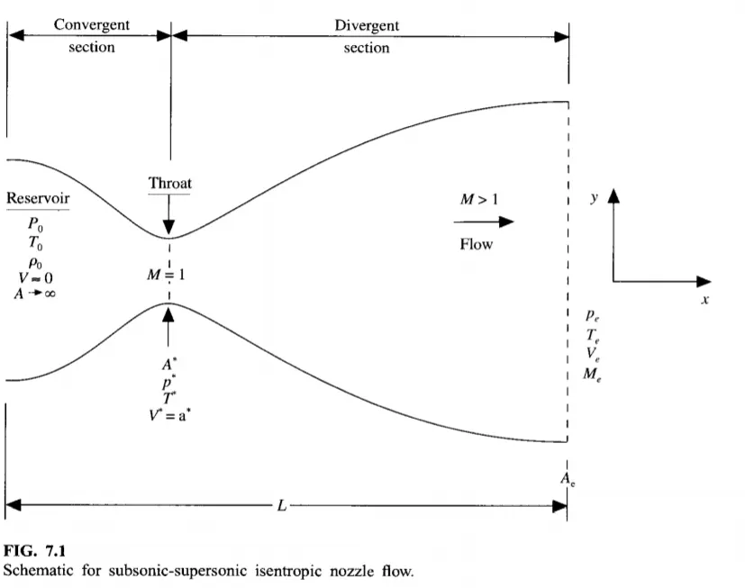
Let us consider a small control volume of the nozzle as shown below.

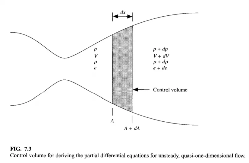
We assume that at a given section, where the cross section area is A, the flow properties are uniform across the section. Hence, although the area of the nozzle changes as a function of distance along the nozzle, X, and therefore in reality the flow field is two dimensional(the flow varies in the two dimensional x-y space), We make the assumption that the flow properties vary only with X; this is tantamount to asuming uniform flow properties across any given cross-section. Such flow is defined as Quasi one dimensional flow.

The governing continuty, momentum and energy equations in terms of non dimensional variables for this quassi one dimensional staedy and isentropc flow can be expressed respectively as:

Non- Conservative Continuty equation:

∂ρ′∂t′=-ρ′(∂V′∂x′)-ρ′V′(∂(lnA′)∂x′)-V′(∂ρ′∂x′)">∂ρ'∂t'=−ρ'(∂V'∂x')−ρ'V'(∂(lnA')∂x')−V'(∂ρ'∂x')∂�′∂�′=-�′(∂�′∂�′)-�′�′(∂(ln�′)∂�′)-�′(∂�′∂�′)

Non- Conservative Momentum equation:

∂V′∂t′=-V′(∂V′∂x′)-(1γ)(∂T′∂x′+T′ρ′(∂ρ′∂x′))">∂V'∂t'=−V'(∂V'∂x')−(1γ)(∂T'∂x'+T'ρ'(∂ρ'∂x'))∂�′∂�′=-�′(∂�′∂�′)-(1�)(∂�′∂�′+�′�′(∂�′∂�′))

Non- Conservative Energy equation:

∂T′∂t′=-V′(∂T′∂x′)-(γ-1)T′[∂V′∂x′+V′∂(lnA′)∂x′]">∂T'∂t'=−V'(∂T'∂x')−(γ−1)T'[∂V'∂x'+V'∂(lnA')∂x']

Conservative Continuty equation:

∂(ρ′A′)∂t′+∂(ρ′A′V′)∂x′=0">∂(ρ'A')∂t'+∂(ρ'A'V')∂x'=0

Conservative Momentum equation:

∂(ρ′A′V′)∂t′+∂[ρ′A′(V′)2+(1γ)ρ′A′]∂x′=(1γ)ρ′(∂A′∂x′)">∂(ρ'A'V')∂t'+∂[ρ'A'(V')2+(1γ)ρ'A']∂x'=(1γ)ρ'(∂A'∂x')∂

Conservative Energy equation:

∂[ρ′(e′γ-1+(γ2)(V′)2)A′]∂t′+∂[ρ′(e′γ-1+(γ2)(V′)2)V′A′+ρ′A′V′]∂x′=0">∂[ρ'(e'γ−1+(γ2)(V')2)A']∂t'+∂[ρ'(e'γ−1+(γ2)(V')2)V'A'+ρ'A'V']∂x'=0

For air at standard conditions, γ=1.4">γ=1.4

These equations are solved by Macormack method using time marching process

Macormack Method:

Let f(x) is the equation to be solved.Then the following steps are followed

i. inital profile

Before the calculation, the initial profile for all the flow field variables which are velocity, density and temperature has to be determined. These are guess values but should be specified with more awareness on the problem.

ii. predector step

(∂fdt)p=f(i+1)-f(i)Δx">(∂fdt)p=f(i+1)−f(i)Δx

iii. solution update

fp=fInitial+(∂f∂t)p⋅Δt">fp=fInitial+(∂f∂t)p⋅Δt

`strong> fp=">fp= Flow field variables calculated after the predictor s`

`strong> fInitial=">fInitial=flow field variable in the initial st`

Δt=">Δt=Δtime step size

iv. Corrector step

(∂fpdt)c=f(i)-f(i-1)Δx">(∂fpdt)c=f(i)−f(i−1)Δ

(∂fdt)avg=0.5((∂fdt)p+(∂fpdt)c)">(∂fdt)avg=0.5((∂fdt)p+(∂fpdt)c)v. Final solution update

fsol=fInitial+(∂f∂t)avg⋅Δt">fsol=fInitial+(∂f∂t)avg⋅Δt

`f_(sol) =`Final solution of the flow field variables for the first time step

Matlab Code :

close all
clear all
clc

L=3;                    %length of nozzle
n=[31 62 93];           %number of grid points
nt=1:1400;              %number of time steps
cfl = 0.5;              %CFL number
for i = 1:length(n)
x=linspace(0,L,n(i));
[mfr_nc,mfr_throat_nc]=non_conservative(L,n(i),nt,cfl);
[mfr_c,mfr_throat_c]=conservative(L,n(i),nt,cfl);
figure(7)
subplot(2,1,1)
plot(nt,mfr_throat_c,'b',nt,mfr_throat_nc,'r','linewidth',1)
xlabel('Time steps (nt)')
ylabel('Mass flow rate')
legend('Conservative form','Non-Conservative form')
title('Mass flow rate using "Non-Conservative form vs Conservative form" at throat point i=16')

subplot (2,1,2)
plot(x,mfr_c,'b',x,mfr_nc,'r','linewidth',1)
xlabel('Length of nozzle')
ylabel('Mass flow rate')
legend('Conservative form','Non-Conservative form')
title('Mass flow rate using "Non-Conservative form vs Conservative form" in the nozzle')

figure(8)
subplot (2,1,1)
plot(nt,mfr_throat_c,'linewidth',1)
hold on
xlabel('Time steps (nt)')
ylabel('Mass flow rate')
legend('@31 nodes','@62 nodes','@93 nodes')
title('Conservative form: Grid independency test at throat point i=16')
subplot (2,1,2)
plot(nt,mfr_throat_nc,'linewidth',1)
hold on
xlabel('Time steps (nt)')
ylabel('Mass flow rate')
legend('@31 nodes','@62 nodes','@93 nodes')
title('Non-Conservative form: Grid independency test at throat point i=16')
figure(9)
subplot (2,1,1)
plot(x,mfr_c,'linewidth',1)
hold on
xlabel('Length of nozzle')
ylabel('Mass flow rate')
legend('@31 nodes','@62 nodes','@93 nodes')
title('Conservative form: Grid independency test along the nozzle')
subplot (2,1,2)
plot(x,mfr_nc,'linewidth',1)
hold on
xlabel('Length of nozzle')
ylabel('Mass flow rate')
legend('@31 nodes','@62 nodes','@93 nodes')
title('Non-Conservative form: Grid independency test along the nozzle')

end

Non-Conservative function:

function [mfr_nc,mfr_throat_nc]=non_conservative(L,n,nt,cfl)


x=linspace(0,L,n);
dx=x(2)-x(1);

% initial conditions rho, a, v, T, mfr, M, p
rho = 1-0.3146*x;
T= 1-0.2314*x;
v=(0.1+1.09*x).*T.^0.5;
a= 1+2.2*(x-1.5).^2;
M= v./(T.^0.5);
mfr = rho.*a.*v;
p=rho.*T;

g = 1.4;

for z=1:31
    u=(T(z))^(1/2);
    dt(z) = cfl*dx/(u + v(z));
end
dt=min(dt);

for i = 1:length(nt)
  %storing initial values
    rho_old = rho;
    T_old = T;
    v_old = v;
  for j=2:n-1
  %predictor step
    drho_dx = (rho(j+1)-rho(j))/dx;
    dv_dx = (v(j+1)-v(j))/dx;
    dT_dx = (T(j+1)-T(j))/dx;
    da_dx = (log(a(j+1))-log(a(j)))/dx;
    drho_dt_p(j) = -rho(j)*dv_dx - rho(j)*v(j)*da_dx - v(j)*drho_dx;        %continuty
    dv_dt_p(j) = -v(j)*dv_dx - (1/g)*(dT_dx + (T(j)/rho(j))*drho_dx);       %momentum
    dT_dt_p(j) = -v(j)*dT_dx - (g-1)*T(j)*(dv_dx + v(j)*da_dx);             %energy
  %updating primitives
    v(j) = v_old(j) + dv_dt_p(j)*dt;
    rho(j) = rho_old(j) + drho_dt_p(j)*dt;
    T(j) = T_old(j) + dT_dt_p(j)*dt;
  %corrector step
    drho_dx = (rho(j)-rho(j-1))/dx;
    dv_dx = (v(j)-v(j-1))/dx;
    dT_dx = (T(j)-T(j-1))/dx;
    da_dx = (log(a(j))-log(a(j-1)))/dx; 
    drho_dt_c(j) = -rho(j)*dv_dx - rho(j)*v(j)*da_dx - v(j)*drho_dx;        %continuity    
    dv_dt_c(j) = -v(j)*dv_dx - (1/g)*(dT_dx + (T(j)/rho(j))*drho_dx);       %momentum
    dT_dt_c(j) = -v(j)*dT_dx - (g-1)*T(j)*(dv_dx + v(j)*da_dx);             %energy
  end
  %average time derivatives
    drho_dt_avg = 0.5*(drho_dt_p + drho_dt_c);
    dv_dt_avg = 0.5*(dv_dt_p + dv_dt_c);
    dT_dt_avg = 0.5*(dT_dt_p + dT_dt_c);
  %final corected values
  for k = 2:n-1
    rho(k) = rho_old(k) + drho_dt_avg(k)*dt;
    v(k) = v_old(k) + dv_dt_avg(k)*dt;
    T(k) = T_old(k) + dT_dt_avg(k)*dt;
  end
  %entry boundary conditions
    v(1) = 2*v(2)-v(3);
  %exit boundary conditions
    v(n) = 2*v(n-1)-v(n-2);
    rho(n) = 2*rho(n-1)-rho(n-2);
    T(n) = 2*T(n-1)-T(n-2);
  %Final update of primitives
    p = rho.*T;
    M= v./T.^0.5;
    error(k) =  abs(v(k)-v(k-1));
    mfr= rho.*a.*v;
  %to find values at throat point
    T_throat(i) = T(16);
    rho_throat(i) = rho(16);
    v_throat(i) = v(16);
    M_throat(i) = M(16);
    p_throat(i) = p(16);
    error_throat(i)=error(16);
    mfr_throat(i)=mfr(16);
    if n==31
for ii=[1:50:201 700]
    if ii==i
       figure(1)
     plot(x,mfr,'linewidth',1)
     hold on
     title ('Non-Conservative form - Variation of Mass flow rate distribution inside the nozzle at different time steps during the time-marching process')
     xlabel('Length of nozzle')
     ylabel('Mass flow rate')   
    elseif i==1400
     plot(x,mfr,'*r')
     legend('@1','@51','@101','@151','@201','@700','@1400') 
    end
end
end
  
end
if n==31
figure(2)
     plot(x,v,'b',x,p,'r',x,T,'k',x,rho,'m',x,M,'g',x,mfr,'c')
     ylim([-0.1 3.7])
     title (sprintf('Time step = %d',i))
     xlabel('Length of nozzle')
     ylabel('Non dimensional parameters')
     legend('Velocity','Pressure','Temperature','Density','Mach number','Mass flow rate','location','northwest')
     title('Non-Conservative form - Steady-state distribution of primitive variables inside the nozzle')

figure (3)
plot(nt,rho_throat)  
hold on
plot(nt,v_throat,'linewidth',1)   
plot(nt,p_throat,'linewidth',1) 
plot(nt,T_throat,'linewidth',1)    
plot(nt,M_throat,'linewidth',1)
plot(nt,mfr_throat,'linewidth',1)
xlabel('Time steps (nt)')
ylabel('Non dimensional parameters')
legend('Density','Velocity','Pressure','Temperature','Mach number','Mass flow rate')
title('Non-Conservative form - Time-wise variation of the primitive variables at throat point i=16')
end
mfr_nc=mfr;
mfr_throat_nc=mfr_throat;
end

Conservative function:

function [mfr_c,mfr_throat_c]=conservative(L,n,nt,cfl)

x=linspace(0,L,n);
dx=x(2)-x(1);

% initial conditions rho, a, v, T, M, mfr, p
for ii=1:length(x)
    if (x(ii)<=0.5)
        rho(ii) = 1;
        T(ii) = 1;
    elseif (x(ii)>0.5) & (x(ii)<=1.5)
        rho(ii) = 1-0.366*(x(ii)-0.5);
        T(ii)= 1-0.167*(x(ii)-0.5);
    elseif (x(ii)>1.5) & (x(ii)<=3.5)
        rho(ii) = 0.634-0.3879*(x(ii)-1.5);
        T(ii)= 0.833-0.3507*(x(ii)-1.5);
    end
end
a= 1+2.2*(x-1.5).^2;     %area
g = 1.4;                 %gamma value
% solution vectors u1, u2, u3
u1 = rho.*a;
u2 = 0.59*ones(1,n);
v=u2./u1;
u3 = u1.*((T./(g-1))+(g/2).*v.^2);

M= v./(T.^0.5);          %mach number
mfr = rho.*a.*v;         %mass flow rate
p=rho.*T;                %pressure


for z=1:31               %to find dt value
u=(T(z))^(1/2);
dt(z) = cfl*dx/(u + v(z));
end
dt=min(dt);

for i = 1:length(nt)
    %storing initial values
    u1_old = u1;
    u2_old = u2;
    u3_old = u3;
   
    for j=2:n-1
   %flux vectors
        f1 = u2;
        f2 = ((u2.^2)./u1)+((g-1)/g)*(u3-((g/2)*(u2.^2)./u1));
        f3 = ((g.*u2.*u3)./u1) - ((g*(g-1)/2)*(u2.^3)./(u1.^2));
   %source term
        j1 = (1/g)*rho(j)*T(j)*((a(j+1)-a(j))/dx);        
   %predictor step
        du1_dt_p(j)= -(f1(j+1)-f1(j))/dx;           %continuity   
        du2_dt_p(j)= -(f2(j+1)-f2(j))/dx + j1;      %momentum
        du3_dt_p(j)= -(f3(j+1)-f3(j))/dx;           %energy
   %updating solution vectors          
        u1(j) = u1_old(j) + du1_dt_p(j)*dt;
        u2(j) = u2_old(j) + du2_dt_p(j)*dt;
        u3(j) = u3_old(j) + du3_dt_p(j)*dt;
   %updating primitives
        rho=u1./a;
        T=(g-1).*(u3./u1-(g/2).*(u2./u1).^2);  
   %updating flux terms
        f1=u2;
        f2=u2.^2./u1+((g-1)/g).*(u3-(g/2)*u2.^2./u1);
        f3=g.*u2.*u3./u1-0.5*g*(g-1).*u2.^3./u1.^2;
   %source term for corrector step
        j2 = (1/g)*(rho(j)*T(j)*(a(j)-a(j-1))/dx);    
   %corrector step
        du1_dt_c(j) = -(f1(j)-f1(j-1))/dx;            %continuity   
        du2_dt_c(j) = -(f2(j)-f2(j-1))/dx + j2;       %momentum
        du3_dt_c(j) = -(f3(j)-f3(j-1))/dx;            %energy
    end
    %average time derivatives
        du1_dt_avg = 0.5*(du1_dt_p + du1_dt_c);
        du2_dt_avg = 0.5*(du2_dt_p + du2_dt_c);
        du3_dt_avg = 0.5*(du3_dt_p + du3_dt_c);
    %final corected values
    for k = 2:n-1
        u1(k) = u1_old(k) + du1_dt_avg(k)*dt;
        u2(k) = u2_old(k) + du2_dt_avg(k)*dt;
        u3(k) = u3_old(k) + du3_dt_avg(k)*dt;
    end
    %entry boundary conditions
        u1(1) = a(1);
        u2(1) = 2*u2(2)-u2(3);
        u3(1) = u1(1)*(T(1)/(g-1) + (g*(u2(1)/u1(1))^2)/2);
    %exit boundary conditions
        u1(n) = 2*u1(n-1)-u1(n-2);
        u2(n) = 2*u2(n-1)-u2(n-2);
        u3(n) = 2*u3(n-1)-u3(n-2);

    %Final update of primitives
        rho = u1./a;
        v = u2./u1;
        T=(g-1).*(u3./u1-(g/2).*(u2./u1).^2);  
        p = rho.*T;
        M= v./T.^0.5;
        error(k) =  abs(v(k)-v(k-1));
        mfr= u2;
  %to find values at throat point
    T_throat(i) = T(16);
    rho_throat(i) = rho(16);
    v_throat(i) = v(16);
    M_throat(i) = M(16);
    p_throat(i) = p(16);
    error_throat(i)=error(16);
    mfr_throat(i)=mfr(16);  
    
if n==31  
    for ii=[1:50:201 700]
    if ii==i
       figure(4)
     plot(x,mfr,'linewidth',1)
     hold on
     title ('Conservative form - Variation of Mass flow rate distribution inside the nozzle at different time steps during the time-marching process')
     xlabel('Length of nozzle')
     ylabel('Mass flow rate')   
    elseif i==1400
     plot(x,mfr,'*r')
     legend('@1','@51','@101','@151','@201','@700','@1400') 
    end
end
end
  

FIgure Explantion :

fig(1) shows Steady state distribution of non dimensional primitive variables at the end of time step. These values of flow field variables obliges the exact values shown in John D. anderson book.

fig(2) shows Time wise variation of primitive variables at throat point i =16. Around the time step of 500 the flow field variables obtained stable solution.

fig(3) shows the variation of mass flow rate distribution inside the nozzle at different time steps during the time marching process. The mass flow rate finally settled at 0.58.

fig(4) shows Steady state distribution of non dimensional primitive variables at the end of time step. These values of flow field variables obliges the exact values shown in John D. anderson book.

fig(5) shows Time wise variation of primitive variables at throat point i =16. Around the time step of 600 the flow field variables obtained stable solution.

fig(6) shows the variation of mass flow rate distribution inside the nozzle at different time steps during the time marching process. The mass flow rate finally settled at 0.56.

fig(7) shows comparision of mass flow rate using both conservative and non-conservative forms.

from subplot 1 : Both the forms reached the stable and exact solution by the end of time steps. But the conservative form obatined the stability at lesser time steps.

from subplot 2 : The difference between both the forms is very less in the nozzle. But the mass flow rate in the conservative form is constant where as in non-conservative form it is varying with 0.582±0.003.