Week 7 - Simulation of a 1D Super-sonic nozzle flow simulation using Macormack Method
%non conservative form
clear all
clc
n=31;
L=3;
x=linspace(0,3,n);
dx=x(2)-x(1);
rhomed=zeros(1,n);
vmed=zeros(1,n);
Tmed=zeros(1,n);
rhoold=1-0.3146*x;
Told=1-0.2314*x;
vold=(0.1+1.09*x).*sqrt(1-0.2314*x);
rhomed=rhoold;
vmed=vold;
Tmed=Told;
A=1+2.2*((x-1.5).^2);
C=0.5;
a=sqrt(1-0.2314*x);
dt=min((C.*dx)./(a+vold));
derrhoold=zeros(1,n);
dervold=zeros(1,n);
derTold=zeros(1,n);
derrhomed=zeros(1,n);
dervmed=zeros(1,n);
derTmed=zeros(1,n);
derrhoavg=zeros(1,n);
dervavg=zeros(1,n);
derTavg=zeros(1,n);
rhonew=zeros(1,n);
vnew=zeros(1,n);
Tnew=zeros(1,n);
gamma=1.4;
nt=(1:1400);
rhothrt=zeros(1,length(nt));
vthrt=zeros(1,length(nt));
Tthrt=zeros(1,length(nt));

for t=(1:length(nt))
for j=2:n-1
    derrhoold(j)=-rhoold(j)*vold(j)*((log(A(j+1))-log(A(j)))/dx)-vold(j)*((rhoold(j+1)-rhoold(j))/dx)-rhoold(j)*((vold(j+1)-vold(j))/dx);
    dervold(j)=-vold(j)*((vold(j+1)-vold(j))/dx)-(1/gamma)*((Told(j+1)-Told(j))/dx)-(1/gamma)*(Told(j)/rhoold(j))*((rhoold(j+1)-rhoold(j))/dx);
    derTold(j)=-vold(j)*((Told(j+1)-Told(j))/dx)-(gamma-1)*Told(j)*((vold(j+1)-vold(j))/dx)-(gamma-1)*Told(j)*vold(j)*((log(A(j+1))-log(A(j)))/dx);
    rhomed(j)=rhoold(j)+derrhoold(j)*dt;
    vmed(j)=vold(j)+dervold(j)*dt;
    Tmed(j)=Told(j)+derTold(j)*dt;
end
for k=2:n-1
derrhomed(k)=-rhomed(k)*vmed(k)*((log(A(k))-log(A(k-1)))/dx)-vold(k)*((rhomed(k)-rhomed(k-1))/dx)-rhomed(k)*((vmed(k)-vmed(k-1))/dx);
dervmed(k)=-vmed(k)*((vmed(k)-vmed(k-1))/dx)-(1/gamma)*((Tmed(k)-Tmed(k-1))/dx)-(1/gamma)*(Tmed(k)/rhomed(k))*((rhomed(k)-rhomed(k-1))/dx);
derTmed(k)=-vmed(k)*((Tmed(k)-Tmed(k-1))/dx)-(gamma-1)*Tmed(k)*((vmed(k)-vmed(k-1))/dx)-(gamma-1)*Tmed(k)*vmed(k)*((log(A(k))-log(A(k-1)))/dx);
end
for p=2:n-1
    derrhoavg(p)=(derrhoold(p)+derrhomed(p))/2;
    dervavg(p)=(dervold(p)+dervmed(p))/2;
    derTavg(p)=(derTold(p)+derTmed(p))/2;
end
for u=2:n-1
    rhonew(u)=rhoold(u)+derrhoavg(u)*dt;
    vnew(u)=vold(u)+dervavg(u)*dt;
    Tnew(u)=Told(u)+derTavg(u)*dt;
    m(u)=rhonew(u)*A(u)*vnew(u);
    P(u)=rhonew(u)*Tnew(u);
    M(u)=vnew(u)/(sqrt(Tnew(u)));
end
vnew(1)=2*vnew(2)-vnew(3);
rhonew(n)=2*rhonew(n-1)-rhonew(n-2);
vnew(n)=2*vnew(n-1)-vnew(n-2);
Tnew(n)=2*Tnew(n-1)-Tnew(n-2);
rhoold=rhonew;
vold=vnew;
Told=Tnew;
rhonew(1)=1;
Tnew(1)=1;
P(1)=1;
P(n)=rhonew(n)*Tnew(n);
m(1)=rhonew(1)*A(1)*vnew(1);
m(n)=rhonew(n)*A(n)*vnew(n);
M(1)=vnew(1)/sqrt(Tnew(1));
M(n)=vnew(n)/sqrt(Tnew(n));
rhothrt(t)=rhonew((n+1)/2);
vthrt(t)=vnew((n+1)/2);
Tthrt(t)=Tnew((n+1)/2);
end
figure(1)
subplot(3,1,1)
plot(nt,rhothrt)
xlabel('timestep')
ylabel('non dimensional density')
title('density convergence')
subplot(3,1,2)
plot(nt,vthrt)
xlabel('timestep')
ylabel('non dimensional velocity')
title('velocity convergence')
subplot(3,1,3)
plot(nt,Tthrt)
xlabel('timestep')
ylabel('non dimensional density')
title('Temperature convergence')
figure(2)
subplot(3,1,1)
plot((x/L),rhonew)
xlabel('non dimensional distance')
ylabel('non dimensional density')
title('density variance')
subplot(3,1,2)
plot((x/L),vnew)
xlabel('non dimensional distance')
ylabel('non dimensional velocity')
title('velocity variance')
subplot(3,1,3)
plot((x/L),Tnew)
xlabel('non dimensional distance')
ylabel('non dimensional temperature')
title('temperature variance')
figure(3)
subplot(2,1,1)
plot((x/L),M)
xlabel('non dimensional distance')
ylabel('Mach number')
title('Mach number variance variance')
subplot(2,1,2)
plot((x/L),P)
xlabel('non dimensional distance')
ylabel('non dimensional pressure')
title('pressure variance')
figure(4)
plot((x/L),m)
xlabel('non dimensional distance')
ylabel('massflowrate ')
title('mass flow rate variance')
%conservative form
clear all
clc
n=31;
L=3;
x=linspace(0,3,n);
dx=x(2)-x(1);
rhoinitial=zeros(1,n);
vintial=zeros(1,n);
Tinitial=zeros(1,n);
A=1+2.2.*(x-1.5).^2;
gamma=1.4;
for i=1:n
    if (x(i)<=0.5)
        rhoinitial(i)=1;
        Tinitial(i)=1;
    elseif (x(i)>0.5)&&(x(i)<=1.5)
        rhoinitial(i)=1-0.366*(x(i)-0.5);
        Tinitial(i)=1-0.167*(x(i)-0.5);
    else
        rhoinitial(i)=0.634-0.3879*(x(i)-1.5);
        Tinitial(i)=0.833-0.3507*(x(i)-1.5);
    end
end
vinitial=0.59./(rhoinitial.*A);
U1initial=rhoinitial.*A;
U2initial=rhoinitial.*A.*vinitial;
U3initial=U1initial.*((Tinitial./(gamma-1))+(gamma/2).*((vinitial).^2));
F1initial=U2initial;
F2initial=((U2initial.^2)./U1initial)+((gamma-1)/gamma)*(U3initial-(gamma/2)*((U2initial.^2)./U1initial));
F3initial=gamma*(U2initial.*U3initial)./(U1initial)-(((gamma)*(gamma-1))/2)*((U2initial.^3)./U1initial.^2);
U1=U1initial;
U2=U2initial;
U3=U3initial;
F1=F1initial;
F2=F2initial;
F3=F3initial;
rho=rhoinitial;
v=vinitial;
T=Tinitial;
C=0.5;
dt=min((C.*dx)./(sqrt(T)+v));
nt=(1:1400);
for t=1:length(nt)
for j=2:n-1
    J2(j)=rho(j)*T(j)*((A(j+1)-A(j))/dx)/gamma;
    derU1(j)=-((F1(j+1)-F1(j))/dx);
    derU2(j)=-((F2(j+1)-F2(j))/dx)+J2(j);
    derU3(j)=-((F3(j+1)-F3(j))/dx);
    U1(j)=U1(j)+derU1(j)*dt;
    U2(j)=U2(j)+derU2(j)*dt;
    U3(j)=U3(j)+derU3(j)*dt;
    rho(j)=U1(j)/A(j);
    T(j)=(gamma-1)*((U3(j)/U1(j))-(gamma/2)*(U2(j)/U1(j))^2);
    F1(j)=U2(j);
    F2(j)=(((U2(j))^2)/U1(j))+((gamma-1)/gamma)*(U3(j)-(gamma/2)*(((U2(j))^2)/U1(j)));
    F3(j)=gamma*(U2(j)*U3(j))/(U1(j))-(((gamma)*(gamma-1))/2)*(((U2(j))^3)/(U1(j))^2);
end
for k=2:n-1
    J2(k)=rho(k)*T(k)*((A(k)-A(k-1))/dx)/gamma;
    dermedU1(k)=-((F1(k)-F1(k-1))/dx);
    dermedU2(k)=-((F2(k)-F2(k-1))/dx)+J2(k);
    dermedU3(k)=-((F3(k)-F3(k-1))/dx);
end
for p=2:n-1
    deravgU1(p)=0.5*(derU1(p)+dermedU1(p));
    deravgU2(p)=0.5*(derU2(p)+dermedU2(p));
    deravgU3(p)=0.5*(derU3(p)+dermedU3(p));
end
for m=2:n-1
    U1(m)=U1initial(m)+(deravgU1(m))*dt;
    U2(m)=U2initial(m)+(deravgU2(m))*dt;
    U3(m)=U3initial(m)+(deravgU3(m))*dt;
    rho(m)=U1(m)/A(m);
    v(m)=(U2(m))/(U1(m));
    T(m)=(gamma-1)*((U3(m))/(U1(m))-(gamma/2)*((v(m))^2));
    massflowrate(m)=rho(m)*A(m)*v(m);
    M(m)=v(m)/(sqrt(T(m)));
    P(m)=rho(m)*T(m);
end
U1(1)=rho(1)*A(1);
U2(1)=2*U2(2)-U2(3);
U3(1)=U1(1)*((T(1)/(gamma-1))+(gamma/2)*((v(1))^2));
U1(n)=2*U1(n-1)-U1(n-2);
U2(n)=2*U2(n-1)-U2(n-2);
U3(n)=2*U3(n-1)-U3(n-2);
U1initial=U1;
U2initial=U2;
U3initial=U3;
F1=U2;
F2=((((U2).^2)./(U1))+((gamma-1)/gamma).*(U3-(gamma/2).*((U2).^2)./U1));
F3=gamma.*(U2.*U3)./(U1)-(((gamma)*(gamma-1))/2).*(((U2).^3)./(U1).^2);
rhothrt(t)=rho((n+1)/2);
vthrt(t)=v((n+1)/2);
Tthrt(t)=T((n+1)/2);
massflowrate(1)=rho(1)*A(1)*v(1);
massflowrate(n)=rho(n)*A(n)*v(n);
M(1)=v(1)/(sqrt(T(1)));
M(n)=v(n)/(sqrt(T(n)));
P(1)=rho(1)*T(1);
P(n)=rho(n)*T(n);
end
figure(1)
subplot(3,1,1)
plot(nt,rhothrt)
xlabel('timestep')
ylabel('non dimensional density')
title('density convergence')
subplot(3,1,2)
plot(nt,vthrt)
xlabel('timestep')
ylabel('non dimensional velocity')
title('velocity convergence')
subplot(3,1,3)
plot(nt,Tthrt)
xlabel('timestep')
ylabel('non dimensional density')
title('Temperature convergence')
figure(2)
subplot(3,1,1)
plot((x/L),rho)
xlabel('non dimensional distance')
ylabel('non dimensional density')
title('density variance')
subplot(3,1,2)
plot((x/L),v)
xlabel('non dimensional distance')
ylabel('non dimensional velocity')
title('velocity variance')
subplot(3,1,3)
plot((x/L),T)
xlabel('non dimensional distance')
ylabel('non dimensional temperature')
title('temperature variance')
figure(3)
subplot(2,1,1)
plot((x/L),M)
xlabel('non dimensional distance')
ylabel('Mach number')
title('Mach number variance variance')
subplot(2,1,2)
plot((x/L),P)
xlabel('non dimensional distance')
ylabel('non dimensional pressure')
title('pressure variance')
figure(4)
plot((x/L),massflowrate)
xlabel('non dimensional distance')
ylabel('massflowrate ')
title('mass flow rate variance')
The number of timesteps were 1400 in the simulation.The following values were calculated for i=16 i.e the throat secton.
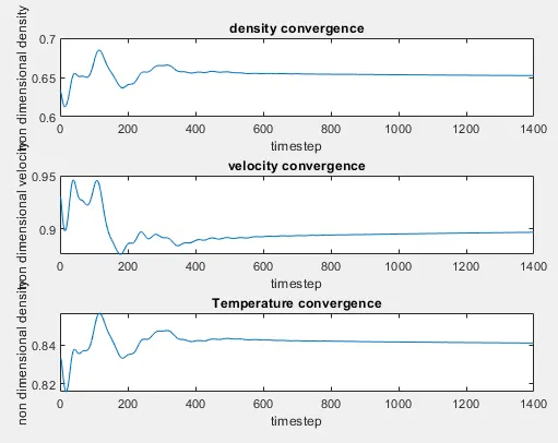
The above represents plot for different convergence of conervative form.
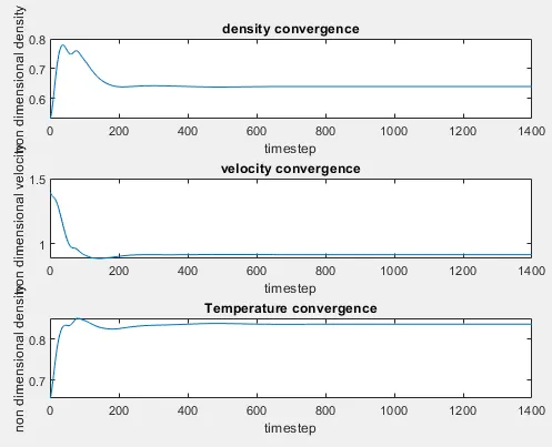
the above is the convergence for non conservative plot.
1.) it can be seen from both of the above plots that the values ocillate a lot this is beause the value of time derivatives initially is quite large.
2.)It can be deduced that the steady state is achieved after 700-800 timsteps when the parameters get constant.
3.)After some time steps the derivatives grow slowly as compared to previous time steps.changin by six orders of magnitude after 1400 time steps. since we have used finite number of time steps it can be deduced that some residuals might be left which is nglected.
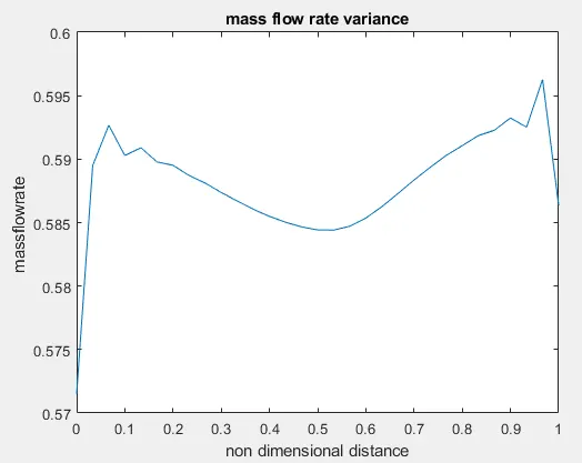
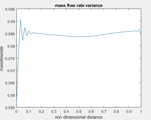
Mass flowrate comparison:
massflowrate of non conservative form:
massflowrate of conservative form:
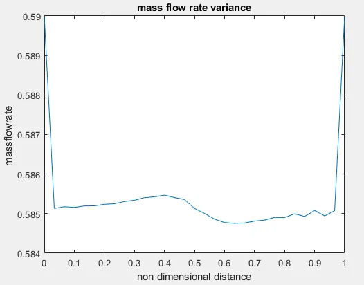
These plots show us that in conservative form of equations the mass flow rate is maintained constant as compared to non conservative form.There are oscilations in case of a non conservative solution.so there is uniform distribution of mass flowrate in case of conservative form.
Faster method:
The time taken to solve conservative form is more than the non conservative form which is due to the reason that in the conservative form we need to calculae U1 U2 U3 to calculate the flux terms . this makes the decoding more complex and hence the nonconservative form is faster.
Grid independence Test:
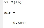
For grid dependance test a parameter mas flow rate is considered at the throatsection after 1400 time steps.
Non conservative form
n=31
n=61
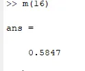
so we see that there is not much difference in value of the non conservative form.
how ever we see that when we increase the number of nodes form 31 to 61 we see that the values are reaching close to the exact situation.
Conservative form:
n=31
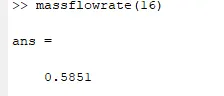
n=61
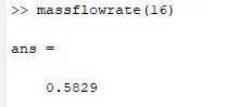
Here also we can see that the solution s=doesnt change on a large magnitude when we g from n=31 to n=61
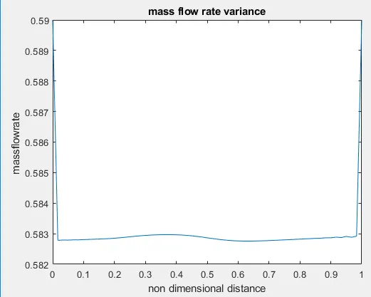
but we can see that the mass flow rate becomes more accurate.
Variance of parameters with nondimensional distance:
non conservative form:
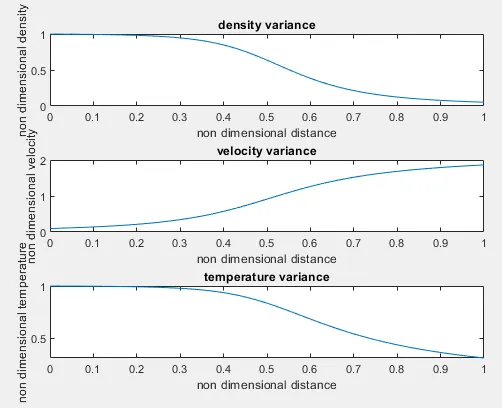
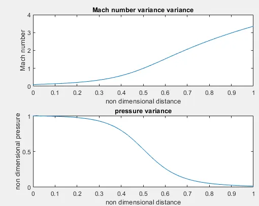
conservative form:
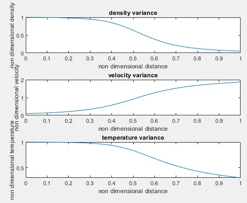
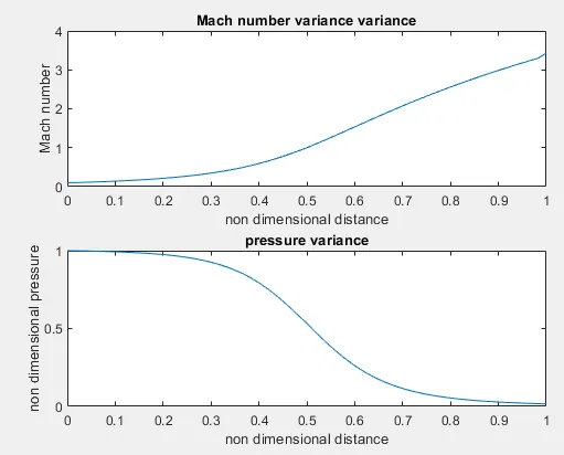
The time step was calculated by using dt=(C*dx)/(a+v) C being the courant number which is assumed to be 0.5.