Simulation of a 1D Super-sonic nozzle flow simulation using Macormack Method
Objective:
- To solve the 1D supersonic nozzle flow equations using the Macro Mack Method.
- Compare the normalized mass flow rate between the conservative forms and non-conservative forms to make suitable conclusions.
- Figure out the minimum number of cycles for which the simulation should be run for convergence.
Plots to be displayed:
- Steady-state distribution of primitive variables inside the nozzle
- Time-waste variation of the primitive variables.
- Variation of Mass flow rate distribution inside the nozzle at different time steps during the time-marching process.
- Comparison of Normalized mass flow rate distributions of both forms.
Introduction:
- Nozzle is used to convert the chemical-thermal energy generated in the combustion chamber into kinetic energy.
- The nozzle converts the low velocity, high pressure, high temperature gas in the combustion chamber into high velocity gas of lower pressure and temperature.
- The one-dimensional in isentropic flow in a convergent-divergent nozzle is a classical textbook problem which can be further solved by using Cascade Theory and 2-d Flow analysis theories.
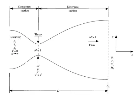
Fig : Basic diagram of 1-D supersonic nozzle flow
- Convergent-Divergent nozzle is designed for attaining speeds that are greater than speed of sound.
- The design of this nozzle came from the area-velocity relation
(dA/dV) =-(A/V)(1-M2)
M is the Mach number (which means ratio of local speed of flow to the local speed of sound)
A is area
V is velocity
Where,
P Pressure
V Velocity
A Area of the nozzle
M Mach Number
MACROMACK METHOD:
This method is employed to solve the governing equations of quasi 1D supersonic nozzle flow rather than the differencing schemes as we have studied earlier. Macro mask method is an explicit finite difference technique which is second order accurate in both time and space. In computational fluid dynamics, the macro mask method is a widely used discretization scheme for the numeri’s solution of hyperbolic partial differential equation. This method essentially uses a predictor step and a corrector step which will be depicted in the code below.
According to the macro mask method, the values of variable at the grid point I,j at the time level t=dt is given as follows,
`upsilon_(i,j)^(t+Deltat)=upsilon_(i,j)^t+((delupsilon)/(delt))_(avg)*Deltat`
Where the average time derivatives is the mean value between time t and t+dt. The average time derivatives is obtained from the predictor-corrector philosophy.
`((delupsilon)/(delt))_(avg)=0.5[((delupsilon)/(delt))_(predicted)+((delupsilon)/(delt))_(corrected)]`
Predictor Step:
In the predictor step, the spatial terms on the right hand side of the equation are replaced by forward differences, The RHS of the equation is known as all values of variables are for time step ‘t’. Next the values of the variables on the LHS is calculated by employing the time marching solution and for the time-step ‘t+dt’ value of the variables at all grid points is obtained.
Considering the following equation for examples,
`((delupsilon)/(delt))=((delrho)/(delx))`
`((delupsilon)/(delt))_(predected)=((rho_(i+1,j)^t-rho_(i,j)^t)/(Deltax)+(rho_(i+1,j)^t-rho_(i,j)^t)/(Deltay))`
`upsilon _(i,j)^(t+Deltat)=upsilon_(i,j)^t+((delupsilon)/(delt))_(predicted)*Deltat`
Corrector Step:
In the corrector step, the spatial terms on the right-hand side are replaced by backward differences. The value of variables on RHS are taken which are obtained in the preditor step for the times step t+dt. Then the corrected time derivative is calculated.
`((delupsilon)/(delt))_(corrected)=(((rho_(i,j)^(t+Deltat)-rho_(i-1,j)^(t+Deltat))/(Deltax))+((rho_(i,j)^(t+Deltat)-rho_(i-1,j)^(t+Deltat))/(Deltay)))`
Now the predicted and corrected value of time derivative is used to calculate the average time derivative which in turn gives the value of the variable at a given point for a time step. The same steps are repeated until the values of variables are obtained for all grid points for a given number of time steps.
In predictor step we are using Forward differencing method for Space terms.
In corrector step we are using Backward differencing method for Space terms.
GOVERNING EQUATIONS:
There are 3 equations that govern the flow of the fluid in the nozzle continuity equation momentum equation and energy equation.
Non-Conservative Equation:
In this type, a control volume is taken into consideration, where the control volume moves with the fluid and properties of the fluid are then taken into consideration.
Continuity Equation:
`-(delrho)/(delt)=-rho((delupsilon)/(delx))-rho*upsilon*(dellnA)/(delx)-upsilon*(delrho)/(delx)`
Momentum Equation:
`-(delupsilon)/(delT)=-upsilon*(delupsilon)/(delx)-(1/rho)*((delT)/(delx)+(t/rho)*(delrho)/(delx))`
Energy Equation:
`-(delT)/(delt)=-upsilon*(delT)/(delx)-(1-rho)*T*((delupsilon)/(delx)+upsilon*(dellnA)/(delx))`
Conservative Equation:
In this type, a control volume is taken into consideration where the control volume is fixed and the flow of the fluid in that control volume is studied.
Continuity Equation:
`-(delrhoA)/(delt)=-(delrhoupsilonA)/(delx)`
Momentum Equation:
`-(delrhoAupsilon)/(delt)=-((del(rhoAupsilon^2+(1/rho)*(rhoA)))/(delx))+(1/(rho))*rho*(delA)/(delx))`
Energy Equation:
`(del(rho*(T/(gamma-1)+(gamma/2)*upsilon^2)*A))/(delt)=-(del(rho*(T/(gamma-1)+(gamma/2)*upsilon^2)*upsilon*A+rhoA*upsilon))/(delx)`
Code for Non-conservative Method:
clear all
close all
clc

n  =  31;
x = linspace(0,3,n)
dx = x(2)- x(1);
gamma = 1.4;
error = 1;
% Initialize Throat
throat = (n + 1)/2;

%Initial Conditions
% Density
rho = 1-0.3146*x;
% Temperature
t = 1-0.2314*x;
% velocity
v = (0.1 + 1.09*x).*t.^0.5;
% Area
a = 1+2.2*(x-1.5).^2;


nt = 900;
dt = 0.01;
error_tolerance = 1e-4;


for k = 1:nt

rho_initial = rho;
v_initial= v;
t_initial = t;

% Predictor_step
for i=2:n-1

dvdx = (v(i+1)-v(i))/dx;
drhodx = (rho(i+1)- rho(i))/dx;
dtdx = (t(i+1)- t(i))/dx;
dlogadx = (log(a(i+1))-log(a(i)))/dx;

% Continuity_equation
drhodt_p (i) = -rho(i)*dvdx -rho(i)*v(i)*dlogadx -v(i)*drhodx ;

% Momentum_equation
dvdt_p(i) = -v(i)*dvdx - (1/gamma)*(dtdx + (t(i)/rho(i))*drhodx);

% Energy_equation
dtdt_p(i) = -v(i)*dtdx - (gamma-1)*t(i)*(dvdx +(v(i)*dlogadx));

% Solution_update
rho(i) = rho(i)+ drhodt_p (i)*dt;
v(i) = v(i) + dvdt_p (i)*dt;
t(i) = t(i) + dtdt_p (i)*dt;

end


% Corrector_method
for j=2:n-1

dvdx = (v (j)-v(j-1))/dx;
drhodx = (rho(j)- rho(j-1))/dx;
dtdx = (t(j)- t(j-1))/dx;
dlogadx = (log(a(j))-log(a(j-1)))/dx;

% Continuity_equation:
drhodt_c (j)= -rho(j)*dvdx -rho(j)*v(j)*dlogadx -v(j)*drhodx;

% Momentum_equation:
dvdt_c(j)= -v(j)*dvdx - (1/gamma)*(dtdx + ((t(j)/rho(j))*drhodx));

% Energy_equation:
dtdt_c(j)= -v(j)*dtdx - (gamma-1)*t(j)*(dvdx +v(j)*dlogadx);


end


drhodt = 0.5*(drhodt_p+drhodt_c);
dvdt =  0.5*(dvdt_p+dvdt_c);
dtdt = 0.5*(dtdt_p+dtdt_c);

% solution_update
for i =2:n-1
rho(i)= rho_initial(i) + drhodt(i)*dt;
v (i)= v_initial (i)+  dvdt(i)*dt;
t(i)= t_initial (i)+ dtdt(i)*dt;
end

%boundary_conditions

%Inlet
rho(1)= 1;
v(1)= 2*v(2)- v(3);
t(1)= 1;

%Outlet
rho(n) = 2*rho(n-1)- rho(n-2);
v(n) = 2*v(n-1)- v(n-2);
t(n) = 2*t(n-1)- t(n-2);

% Pressure
P = rho.*t;

% Mach_number
M =  (v./(t).^0.5);

% Mass_flow_rate
m =  rho.*v.*a;


rho_throat (k)=  rho(throat);
v_throat (k)=  v(throat);
t_throat(k)=  t(throat);
P_throat(k) =  P(throat);
M_throat (k)=  M(throat);
m_throat (k)=  m(throat);


figure(1)
hold all
grid on

if k == 1
plot(x,m,'g');
elseif k == 50
plot(x,m,'m');
elseif k == 100
plot(x,m,'y');
elseif k == 150
plot(x,m,'b');
elseif k == 200
plot(x,m,'r');
elseif k == 700
plot(x,m,'c');

xlabel('Distance through nozzle')
ylabel('Mass flow rate')
legend ('1','50','100','150','200','700');
title(' Mass flow rate at different time step Non conservative form')

end

end

figure(2)
subplot(2,3,1)
plot(x,rho,'r');
xlabel ('Length of nozzle')
ylabel ('Density')
title('Density Non conservative form')
grid minor

subplot(2,3,2)
plot(x,t,'b');
xlabel ('Length of nozzle')
ylabel ('Temperature ')
title('Temperature Non conservative form')
grid minor

subplot(2,3,3)
plot(x,P,'g');
xlabel ('Length of nozzle')
ylabel ('Pressure ')
title('Pressure Non conservative form')
grid minor

subplot(2,3,4)
plot(x,v,'m');
xlabel ('Length of nozzle')
ylabel ('velocity')
title('velocity Non conservative form')
grid minor

subplot(2,3,5)
plot(x,M, 'y');
xlabel ('Length of nozzle')
ylabel ('Mach number ')
title('Mach number Non conservative form')
grid minor

subplot(2,3,6)
plot(x,m,'k');
xlabel ('Length of nozzle')
ylabel ('Mass flow rate ')
title('Mass flow rate Non conservative form')
grid minor

figure (3)
subplot(6,1,1)
plot(1:nt,rho_throat,'r')
xlabel ('Time steps')
ylabel ('Density')
title('Variation of Density at the nozzle throat Non conservative form')
grid minor

subplot(6,1,2)
plot(1:nt,t_throat,'g')
xlabel ('Time steps')
ylabel ('Temperature ')
title('Variation of Temperature at the nozzle throat Non conservative form')
grid minor

subplot(6,1,3)
plot(1:nt,P_throat,'m')
xlabel ('Time steps')
ylabel ('Pressure ')
title('Variation of Pressure at the nozzle throat Non conservative form')
grid minor

subplot(6,1,4)
plot(1:nt,v_throat,'b')
xlabel ('Time steps')
ylabel ('Velocity')
title('Variation of Velocity at the nozzle throat Non conservative form')
grid minor

subplot(6,1,5)
plot(1:nt,M_throat,'k' )
xlabel ('Time steps')
ylabel ('Mach number ')
title('Variation of Mach number at the nozzle throat Non conservative form')
grid minor

subplot(6,1,6)
plot(1:nt,m_throat,'y')
xlabel ('Time steps')
ylabel ('Mass flow rate ')
title('Variation of Mass flow rate at the nozzle throat Non conservative form')
grid minor

figure(4)
hold all
grid on
plot(x,m,'c')
plot(x,linspace (0.579,0.579,n),'g')
xlabel ('Non dimensional Length' )
ylabel ('Mass flow rate ')
legend ('Mass flow rate in Non conservative form','Analytical solution')
Convservative Form Code:
clear all
close all
clc

n  =  31;
x = linspace(0,3,n)
dx = x(2)- x(1);
gamma = 1.4;
error = 1;
% Initialize Throat
throat = (n + 1)/2;

nt = 900;
dt = 0.01;
error_tolerance = 1e-4;

for i =1:n
    if x(i)>=0 && x(i)<0.5
    rho(i) = 1;
    t(i) = 1;

    elseif x(i)>=0.5 && x(i)<1.5
    rho(i)= 1-(0.366*(x(i)-0.5));
    t(i) = 1-(0.167*(x(i)-0.5));
    elseif x(i)>=1.5 && x(i)<3.5
    rho(i)= 0.634-(0.3879*(x(i)-015));
    t(i) = 0.833-(0.3507*(x(i)-1.5));
    end
end


%Initial Conditions
% Density
rho = 1-0.3146*x;
% Temperature
t = 1-0.2314*x;

% Area
a = 1+2.2*(x-1.5).^2;

% velocity
v = 0.59./(rho.*a);

P = rho.*t;

% Defining elements of solution vector U,
U1 = rho.*a;
U2 = rho.*a.*v;
U3 = rho.*a.*((t./(gamma-1))+((gamma/2).*(v.^2)));

%Outer time loop
for k = 1:nt

U1_old = U1;
U2_old = U2;
U3_old = U3;

% Defining elements of Flux vector F,
F1 = U2;
F2 = ((U2.^2)./(U1))+ ((gamma-1)/gamma).*(U3 - (0.5*gamma.*U2.^2)./U1);
F3 = (gamma.*U2.*U3./U1)- ((0.5*gamma*(gamma-1).*U2.^3)./(U1.^2));


% Predictor_method

for i = 2:n-1

dF1dx = (F1(i+1)-F1(i))/dx;
dF2dx = (F2(i+1)-F2(i))/dx;
dF3dx = (F3(i+1)-F3(i))/dx;
dadx = (a(i+1)- a(i))/dx;

% continuity equation:
dU1dt_p(i) = -dF1dx;
% momentum equation:
J2(i) = (1/gamma).*rho(i).*t(i).*((a(i+1) - a(i))/dx);
dU2dt_p(i) =-dF2dx + J2(i); %Where J is the source term.
% Energy equation:
dU3dt_p (i) = -dF3dx;

% Solution Update;
U1(i) = U1(i) + dU1dt_p(i)*dt;
U2(i) = U2(i) + dU2dt_p(i)*dt;
U3(i) = U3(i) + dU3dt_p(i)*dt;

end

% updating values,
P = rho.*t; % Non dimensional pressure
v = U2./U1;
rho = U1./a;
t = (gamma-1).*((U3 ./U1)- ((gamma./2).*(v .^2)));

% Updating elements of Flux vector F,
F1 = U2;
F2 = ((U2.^2)./(U1))+ ((gamma-1)/gamma).*(U3-(0.5*gamma.*U2.^2)./U1);
F3 = (gamma.*U2.*U3./U1)- ((0.5.*gamma.*(gamma-1).*U2.^3)./(U1.^2));

% Corrector_method

for j = 2:n-1

dF1dx = (F1(j)-F1(j-1))/dx;
dF2dx = (F2(j)-F2(j-1))/dx;
dF3dx = (F3(j)-F3(j-1))/dx;


% continuity equation:
dU1dt_c(j)= -dF1dx;

% momentum equation:
J2(j)=(1/gamma).*rho(j).*t(j).*((a(j)- a(j-1))/dx);

dU2dt_c(j)= -dF2dx + J2(j);

% Energy equation:
dU3dt_c(j)= -dF3dx;


end


% Compute the average time derivative
dU1dt_average =  0.5.*(dU1dt_p + dU1dt_c);
dU2dt_average =  0.5.*(dU2dt_p + dU2dt_c);
dU3dt_average =  0.5.*(dU3dt_p + dU3dt_c);

% Updating dependent variables U1,U2&U3.
for l = 2:n-1
U1(l) = U1_old(l)+dU1dt_average(l)*dt;
U2(l) = U2_old(l)+dU2dt_average(l)*dt;
U3(l) = U3_old(l)+dU3dt_average(l)*dt;
end

% Applying boundary conditions,

%Inlet
U2(1)=  2*U2(2)- U2(3);


%Outlet
U1(n) = 2*U1(n-1)-U1(n-2);
U2(n) = 2*U2(n-1)-U2(n-2);
U3(n) = 2*U3(n-1)-U3(n-2);


% Updating the flow field variables,
rho = U1./a;
v = U2./U1;
T = (gamma-1).*((U3 ./U1)- ((gamma*v.^2)/2));


% Pressure
P = rho.*t;

% Mach_number
M =  (v./(t).^0.5);

% Mass_flow_rate
m =  rho.*v.*a;


rho_throat(k)=  rho(throat);
v_throat(k)=  v(throat);
t_throat(k)=  t(throat);
P_throat(k) =  P(throat);
M_throat(k)=  M(throat);
m_throat(k)=  m(throat);


figure(1)
hold all
grid on

if k == 1
plot(x,m,'g');
elseif k == 50
plot(x,m,'m');
elseif k == 100
plot(x,m,'y');
elseif k == 150
plot(x,m,'b');
elseif k == 200
plot(x,m,'r');
elseif k == 700
plot(x,m,'c');

xlabel('Distance through nozzle')
ylabel('Mass flow rate')
legend ('1','50','100','150','200','700');
title(' Mass flow rate at different time step Conservative form')

end

end

figure(2)
subplot(2,3,1)
plot(x,rho,'r');
xlabel ('Length of nozzle')
ylabel ('Density')
title('Density conservative form')
grid minor

subplot(2,3,2)
plot(x,t,'b');
xlabel ('Length of nozzle')
ylabel ('Temperature ')
title('Temperature conservative form')
grid minor

subplot(2,3,3)
plot(x,P,'g');
xlabel ('Length of nozzle')
ylabel ('Pressure ')
title('Pressure conservative form')
grid minor

subplot(2,3,4)
plot(x,v,'m');
xlabel ('Length of nozzle')
ylabel ('velocity')
title('velocity conservative form')
grid minor

subplot(2,3,5)
plot(x,M,'y');
xlabel ('Length of nozzle')
ylabel ('Mach number ')
title('Mach number conservative form')
grid minor

subplot(2,3,6)
plot(x,m,'k');
xlabel ('Length of nozzle')
ylabel ('Mass flow rate')
title('Mass flow rate conservative form')
grid minor

figure (3)
subplot(6,1,1)
plot(1:nt,rho_throat,'r')
xlabel ('Time steps')
ylabel ('Density')
title('Variation of Density at the nozzle throat conservative form')
grid minor

subplot(6,1,2)
plot(1:nt,t_throat,'g')
xlabel ('Time steps')
ylabel ('Temperature ')
title('Variation of Temperature at the nozzle throat conservative form')
grid minor

subplot(6,1,3)
plot(1:nt,P_throat,'m')
xlabel ('Time steps')
ylabel ('Pressure ')
title('Variation of Pressure at the nozzle throat conservative form')
grid minor

subplot(6,1,4)
plot(1:nt,v_throat,'b')
xlabel ('Time steps')
ylabel ('Velocity')
title('Variation of Velocity at the nozzle throat conservative form')
grid minor

subplot(6,1,5)
plot(1:nt,M_throat,'k')
xlabel ('Time steps')
ylabel ('Mach number ')
title('Variation of Mach number at the nozzle throat conservative form')
grid minor

subplot(6,1,6)
plot(1:nt,m_throat,'y')
xlabel ('Time steps')
ylabel ('Mass flow rate ')
title('Variation of Mass flow rate at the nozzle throat conservative form')
grid minor

figure(4)
hold all
grid on
plot(x,m,'c')
plot(x,linspace (0.579,0.579,n),'g')
xlabel ('Non dimensional Length' )
ylabel ('Mass flow rate ')
legend ('Mass flow rate in conservative form','Analytical solution')
Results/Plots:
Mass Flow Rate Comparison:
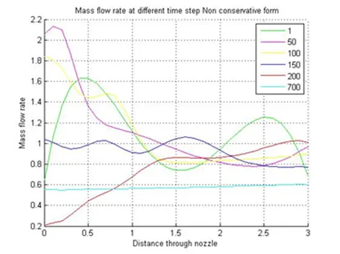
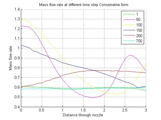
The mass flow rate at various time steps for a non-conservative method is observed that, until 50th timestep it is noticed that the mass flow rate is fluctuating extremely whereas after the 100th or 150th time steps suddenly is started dropping down due to the transient variation of the flow field variables.
In further stages after 200th time steps, the mass flow distribution started settling down slowly and at 700 time step its clearly observed that it started following a straight horizontal path.
Comparing the conservative method to the nonconservative method is is noted that, there were no much deflections in the low as compared to non-conservative method in the initial methods. It too little more time to stabilize the flow through the nozzle.
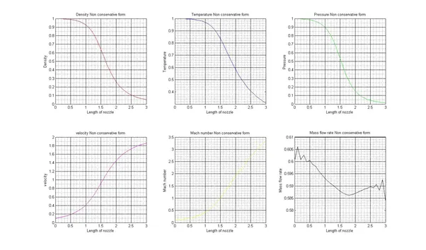
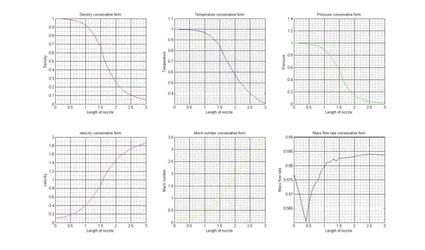
Variation of variables across the length of nozzle for Non-conservative and conservative forms:
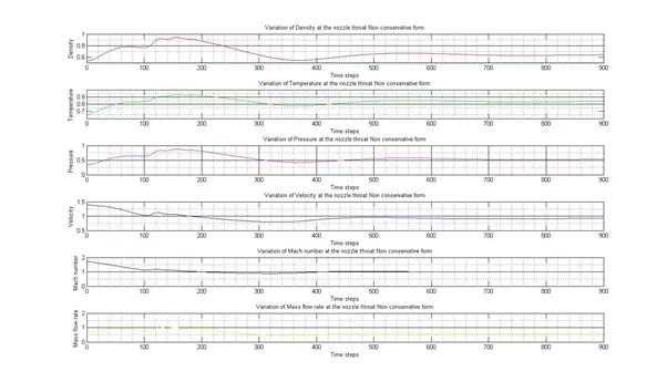
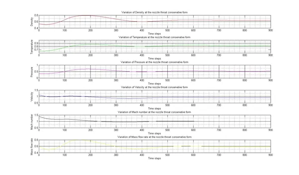
Variation in flow properties w.r.t time steps at throat:
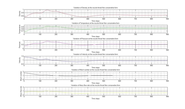
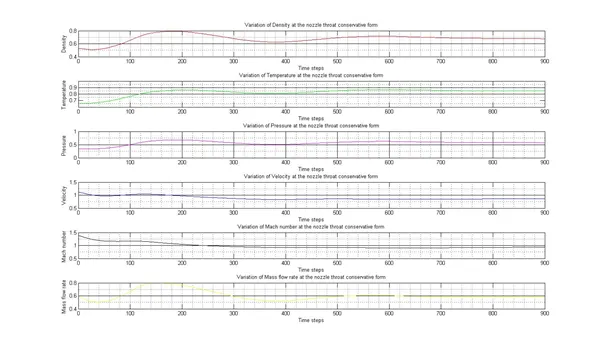
It is observed that the variation is much lower for the conservative form as compared to non-conservative form. Initial there are very small deviations but immediately they will come to stable position.
The variation of mass flow rate along the length of the nozzle is comparatively less for conservative form, Whereas for the non-conservative flow during inlet and outlet some disturbances were observed i.e. we can see the oscillations at inlet and out flow for non-conservative form.
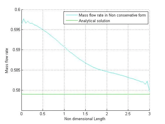
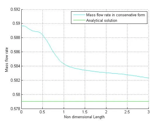
Comparing the mass flow rate of non-conservative form with the analytical solution and the mass flow rate of conservative form with the analytical solution.
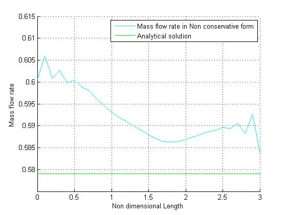
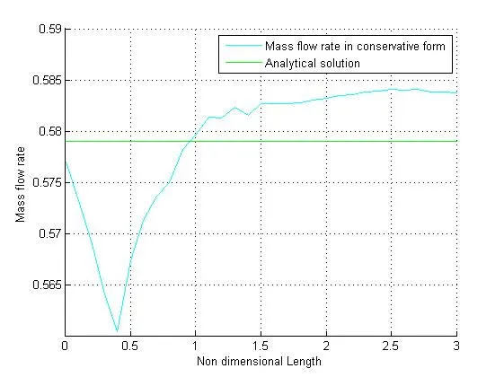
For the mass flow rate of the non-conservative form, it is observed that there is too much of disturbances in the flow at inlet and outlet boundaries. When considering the conservative form, initially there is a huge drop and slowly is started the following the constant path.
Grid Dependency:
The solution is said to be grid independent if the solution has no effect even when the number o grid points are increased once the stable solution is achieved.
In our case let us double the grid points to n=61 and accordingly the dt must be changed.
This can be done by time step calculation from courant number at each grid and the least one is taken.
So, for n=61 we should have nt=2800 time step, Therefore for grid independency it should repeat the exact solution at n=31.
The above code written with changed n values and nt as n=61 and nt=2800 to show the solution is grid independent. The results are displayed for the code with changed value for n and nt.
Output For N=61 Grid Points:
Variation of variables across the length of nozzle for non-conservative and conservative forms:
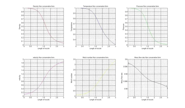
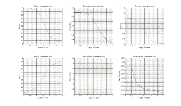
Variation of variable w.r.to time steps at the Nozzle throat for non-conservative and conservative forms:
Comparing the mass flow rate of Non- conservative form with the analytical solution and the mass flow rate of conservative form with the analytical solution:
Conclusion:
In summary, for the given flow problem, we cannot establish a clear superiority of the conservation form of the governing equations over the non - conservative form. Form all our previous discussions, we can only make the following observations:
- The conservation form yields a better mass flow distribution. The conservation form simply does a better job of conserving mass.
- The non - conservative form leads to smaller residuals. The amount by which the residuals decay is often used as an index of “quality” of the numerical algorithm. In this sense, the non - conservation form does a better job.
- There is no clear superiority of either form in terms of accuracy of the results. The non - conservative form seems to produce slightly more accurate results for the primitive variables, and the conservation form seems to produce slightly more accurate results for the flux variables. The results in either case is certainly satisfactory.
- Comparing the amount of calculational effort to achieve a solution, as reflected in our extended discussions, we note that the solution of the conservation form requires marginally more work. Most of this is due to the need to decode the primitive variables from the flux variables, such decoding is not necessary when you are solving the non - conservative form.