Week 7 - Simulation of a 1D Super-sonic nozzle flow simulation using Macormack Method

Aim:

• To simulate the isentropic flow through a quasi 1D subsonic-supersonic nozzle
• To derive the conservation and non conservation forms of the governing equation and solve them using MacCormack's technique
• To plot the steady state distrubution of primitive variables inside the nozzle, Time wise variation, and mass flow rate

Subsonic -Supersonic nozzle

The subsonic-supersonic nozzle consists of two section namely convergent and divergent section  of length L seperated by throat region

Theory

 For fluid flow through nozzle,the flow field variables are expressed in non dimensional form. the expression of fluid flow through non dimensional form is as follows

T'=`T/T^0`

`rho=rho/rho^0`

V'=`V/(aunderset0`

where `aunderset 0` is speed of sound

`aunderset0`=`sqrtgammarT`

t'=t/L/`aunderset0`

A'=A/`Aoverset*`

`Aoverset*`=Throat area

Boundary Condetion

Flow is unsteady,inviscid which is governed by hyperbolic equations.For 1D unsteady flow , there exists 2 real charecteristic lines for apoint in a plane.Boundary condition is provided at the domain of dependence.

Nozzle area A=1+2.2*`(x-1.5)^2`

pressurep=`rho*T`

Machn no=V/`sqrtT`

Mass flow rate=`rho*A*V`

Plots

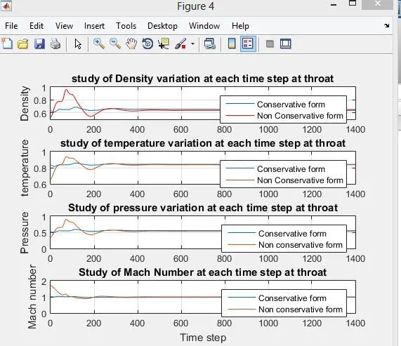
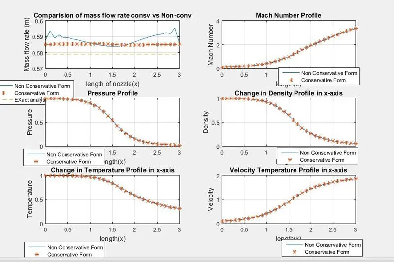
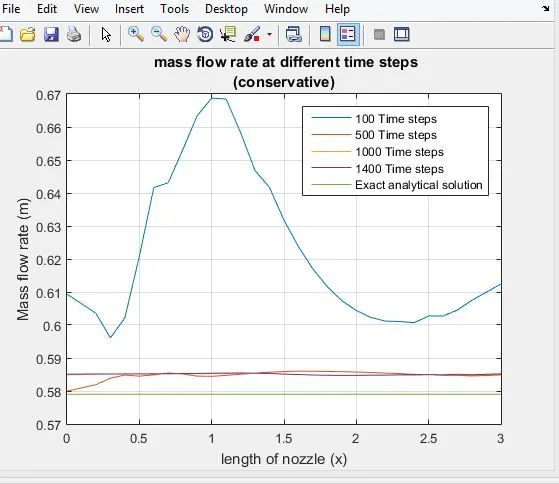
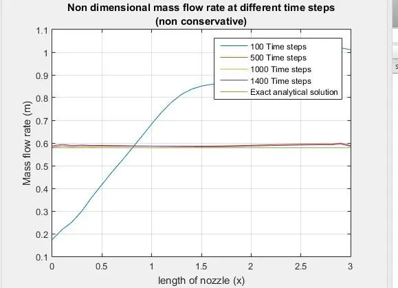
Explanation

• Conservative form of mass flow rate  gives better results  than the non conservative form
• The simulation time  required  for the conservative form is lesss compare to the non conservative form. There fore convergence rate is faster in conservative form

Conclusion

• Using MATLAB , the isentopic flow through a quasi 1D subsonic-suoersonic nozzle was simulated
• The conservation and non conservation forms of the governing equations were solved using McCormack's technique

Distribution of primitive variables , mass flow rate through the nozzle and time-wise variations of primitive variables at throat were plotted for both of the form

clear all
close all
clc

% grid 
n=31;
 
x=linspace(0,3,n);
dx=x(2)-x(1);
% Nozzle area
A=1+2.2*(x-1.5).^2;
%gamma
gamma=1.4;
%Time steps
nt=1400;
C=0.5;

%throat Values
throat=((n-1)/2)+1;

%non conservativw form function
tic
[V,rho,T,m,M,P,V_t,rho_t,T_t,m_t,M_t,P_t]=non_consv(x,gamma,dx,A,n,nt,C,throat);
non_consv_form=toc;
%consevative form
tic
[Vc,rhoc,Tc,mc,Mc,Pc,V_tc,rho_tc,T_tc,m_tc,M_tc,P_tc]=consv(x,gamma,dx,A,n,nt,C,throat);
consv=toc;
%plots for conservative vs non conservative
%Mass Flow rate
figure(3)
subplot(3,2,1)
plot(x,m)
hold on
plot(x,mc,'*')

%Analytical solution  rho*A*V=0.579
plot(x,linspace(0.579,0.579,n),'--')
xlabel('length of nozzle(x)');
ylabel('Mass flow rate (m)');
legend('Non Conservative Form','Conservative Form','EXact analytical solution');
title('Comparision of mass flow rate consv vs Non-conv');
grid on

%Mach number
subplot(3,2,2)
plot(x,M);
hold on
plot(x,Mc,'*');
grid on;
xlabel('length(x)');
ylabel('Mach Number');
legend('Non Conservative Form','Conservative Form','EXact analytical solution');
title('Mach Number Profile')


%Pressure
subplot(3,2,3)
plot(x,P);
hold on
plot(x,Pc,'*');
grid on;
xlabel('length(x)');
ylabel('Pressure');
legend('Non Conservative Form','Conservative Form','EXact analytical solution');
title('Pressure Profile')

%Density
subplot(3,2,4)
plot(x,rho);
hold on
plot(x,rhoc,'*');
grid on;
xlabel('length(x)');
ylabel('Density');
legend('Non Conservative Form','Conservative Form','EXact analytical solution');
title('Change in Density Profile in x-axis')

%Temperature
subplot(3,2,5)
plot(x,T);
hold on
plot(x,Tc,'*');
grid on;
xlabel('length(x)');
ylabel('Temperature');
legend('Non Conservative Form','Conservative Form','EXact analytical solution');
title('Change in Temperature Profile in x-axis')

%velocity
subplot(3,2,6)
plot(x,V);
hold on
plot(x,Vc,'*');
grid on;
xlabel('length(x)');
ylabel('Velocity');
legend('Non Conservative Form','Conservative Form','EXact analytical solution');
title('Velocity Temperature Profile in x-axis')

%Variation of flow proparties at throat
figure(4)
subplot(4,1,1);
plot(1:nt,rho_tc);
hold on
plot(1:nt,rho_t,'color','r');

grid on
ylabel('Density');
legend('Conservative form','Non Conservative form');
title('study of Density variation at each time step at throat');


figure(4)
subplot(4,1,2);
plot(1:nt,T_tc);
hold on
plot(1:nt,T_t);

grid on
ylabel('temperature');
legend('Conservative form','Non Conservative form');
title('study of temperature variation at each time step at throat');

subplot(4,1,3);
plot(1:nt,P_tc);
hold on 
plot(1:nt,P_t);
grid on
ylabel('Pressure');
legend('Conservative form','Non conservative form');
title('Study of pressure variation at each time step at throat');


subplot(4,1,4);
plot(1:nt,M_tc);
hold on 
plot(1:nt,M_t);
grid on
xlabel('Time step')
ylabel('Mach number');
legend('Conservative form','Non conservative form');
title('Study of Mach Number at each time step at throat');




%Function
function [Vc,rhoc,Tc,mc,Mc,Pc,V_tc,rho_tc,T_t,m_tc,M_tc,P_t]=consv(x,gamma,dx,A,n,nt,C,Throat)
for i=1:n
    if (x(i)>=0 && x(i)<=0.5)
        rhoc(i)=1;
        Tc(i)=1;
    elseif(x(i)>=0.5 && x(i)<=1.5)
            rhoc(i)=1-0.366*(x(i)-0.5);
            Tc(i)=1-0.167*(x(i)-0.5);
    elseif (x(i)>=1.5 && x(i)<=3.5)
        rhoc(i)=0.634-0.3879*(x(i)-1.5);
        Tc(i)=0.833-0.3507*(x(i)-1.5);
    end
end

%Calculating non dimensional numbers
Vc=0.59./(rhoc.*A);
Pc=rhoc.*Tc;

%Time step
dt=min(C.*dx./(sqrt(Tc)+Vc));

%solution vector parameters

U1=rhoc.*A;
U2=rhoc.*A.*Vc;
U3=rhoc.*A.*((Tc./(gamma-1))+((gamma/2).*(Vc.^2)));

for k=1:nt
    
    U1_old=U1;
    U2_old=U2;
    U3_old=U3;
    
    
    %Flux terms
    F1=U2;
    F2=((U2.^2)./U1)+(((gamma-1)/gamma)*(U3-((gamma/2)*((U2.^2)./U1))));
    F3=((gamma*U2.*U3)./U1)-(gamma*(gamma-1)*(U2.^3))./(2*U1.^2);
    
    %Predictor
    for i=2:n-1
        
        df1dx(i)=(F1(i+1)-F1(i))/dx;
        df2dx(i)=(F2(i+1)-F2(i))/dx;
        df3dx(i)=(F3(i+1)-F3(i))/dx;
        
        % Updating the value of j2
        dadx(i)=(A(i+1)-A(i))/dx;
        J2(i)=(1/gamma)*(rhoc(i)*Tc(i))*dadx(i);
        
        %continuity equation
        du1dt_p(i)=-df1dx(i);
        
        %Momentum equation
        du2dt_p(i)=-df2dx(i)+J2(i);
        
        %Energy equation
        du3dt_p(i)=-df3dx(i);
        
        
        %solution update
        U1(i)=U1(i)+du1dt_p(i)*dt;
        U2(i)=U2(i)+du2dt_p(i)*dt;
        U3(i)=U3(i)+du3dt_p(i)*dt;
    end
    
    % updating value
    rhoc=U1./A;
    Vc=U2./U1;
    Tc=(gamma-1)*((U3./U1)-((gamma*Vc.^2)/2));
    
    %updating flux for the error
    F1=U2;
    F2=((U2.^2)./U1)+(((gamma-1)/gamma)*(U3-(gamma*U2.^2)./(2*U1)));
    F3=((gamma*U2.*U3)./U1)-(gamma*(gamma-1)*(U2.^3))./(2*U1.^2);
    
    %Corrector method
    for i=2:n-1
        
        df1dx(i)=(F1(i)-F1(i-1))/dx;
        df2dx(i)=(F2(i)-F2(i-1))/dx;
        df3dx(i)=(F3(i)-F3(i-1))/dx;
        
        %updating value of j2
        dadx(i)=(A(i)-A(i-1))/dx;
        J2(i)=(1/gamma)*(rhoc(i)*Tc(i))*dadx(i);
        
        %Continuity eqyation
        du1dt_c(i)=-df1dx(i);
        
        %momentum equation
        du2dt_c(i)=-df2dx(i)+J2(i);
        
        %Energu equation
        du3dt_c(i) = -df3dx(i);
    end
        
        
        
        
        
    %average value
    
    du1dt=0.5*(du1dt_p + du1dt_c);
    du2dt=0.5*(du2dt_p + du2dt_c);
    du3dt=0.5*(du3dt_p +du3dt_c);
    
    %solution vector
    for i=2:n-1
        U1(i)=U1_old(i) + du1dt(i)*dt;
        U2(i)=U2_old(i) + du2dt(i)*dt;
        U3(i)=U3_old(i) + du3dt(i)*dt;
    end
    %boundary condetion
    U1(1)=rhoc(1)*A(1);
    U2(1)=2*U2(2)-U2(3);
    Vc(1)=U2(1)/U1(1);
    U3(1)=U1(1)*((Tc(1)/(gamma-1))+((gamma/2)*Vc(1)^2));
    
    %outlet
    U1(n)=2*U1(n-1)-U1(n-2);
    U2(n)=2*U2(n-1)-U2(n-2);
    U3(n)=2*U3(n-1)-U3(n-2);
    %primitive terms
    rhoc=U1./A;
    Vc=U2./U1;
    Tc=(gamma-1)*((U3./U1)-((gamma*Vc.^2)/2));
    
    %mach,mass,pressure
    mc=rhoc.*Vc.*A;
    Mc=Vc./sqrt(Tc);
    Pc=rhoc.*Tc;
    
    %throat value
    rho_tc(k)=rhoc(Throat);
    T_t(k)=Tc(Throat);
    P_t(k)=Pc(Throat);
    M_tc(k)=Mc(Throat);
    V_tc(k)=Vc(Throat);
    m_tc(k)=mc(Throat);
    
     figure(2)
    if k==100
        plot(x,mc)
        hold on
        grid on
    elseif k==500
            plot(x,mc)
    elseif k==1000
                plot(x,mc)
    elseif k==1400
                    plot(x,mc)
                end
            end
            plot(x,linspace(0.579,0.579,n),'-')
            xlabel('length of nozzle (x)');
            ylabel('Mass flow rate (m)');
            title({' mass flow rate at different time steps';'(conservative)'});
            legend({'100 Time steps','500 Time steps','1000 Time steps','1400 Time steps','Exact analytical solution'});
        end
        
        %Function
function [V,rho,T,m,M,P,V_t,rho_t,T_t,m_t,M_t,P_t]=non_consv(x,gamma,dx,A,n,nt,C,throat)

%Initial condition
rho=1-0.3146*x;
T=1-0.2314*x;
V=(0.1+1.09*x).*T.^0.5;

%Calculating time steps
dt=min(C.*dx./(sqrt(T)+(V)));


%Outer Time loop
for k=1:nt
    rho_old=rho;
    T_old=T;
    V_old=V;
    
    %Predictor step
    
    for i=2:n-1
        dvdx_p=(V(i+1)-V(i))/dx;
        dtdx_p=(T(i+1)-T(i))/dx;
        drhodx_p=(rho(i+1)-rho(i))/dx;
        dlog_adx_p=(log(A(i+1))-log(A(i)))/dx;
        
        %continuity equation
        drhodt_p(i)=-(rho(i)*dvdx_p)-(rho(i)*V(i)*dlog_adx_p)-(V(i)*drhodx_p);
        %momentum eq
        dvdt_p(i)=-(V(i)*dvdx_p)-(1/gamma)*(dtdx_p+(T(i)/rho(i))*drhodx_p);
        %Energy equation
        dtdt_p(i)=-(V(i)*dtdx_p)-(gamma-1)*(T(i))*(dvdx_p+(V(i)*dlog_adx_p));
        
        %Update soln
        rho(i)=rho(i)+drhodt_p(i)*dt;
        V(i)=V(i)+dvdt_p(i)*dt;
        T(i)=T(i)+dtdt_p(i)*dt;
    end
    
   
    
    for j=2:n-1
        
        dvdx_c=(V(j)-V(j-1))/dx;
        dtdx_c=(T(j)-T(j-1))/dx;
        drhodx_c=(rho(j)-rho(j-1))/dx;
        dlog_adx_c=(log(A(j))-log(A(j-1)))/dx;
        
         %continuity equation
        drhodt_c(j)=-(rho(j)*dvdx_c)-(rho(j)*V(j)*dlog_adx_c)-(V(j)*drhodx_c);
        %momentum eq
        dvdt_c(j)=-(V(j)*dvdx_c)-(1/gamma)*(dtdx_c+(T(j)/rho(j))*drhodx_c);
        %Energy equation
        dtdt_c(j)=-(V(j)*dtdx_c)-(gamma-1)*(T(j))*(dvdx_c+(V(j)*dlog_adx_c));
    end
        
        
       %avg time value
       drhodt_avg = 0.5*(drhodt_p + drhodt_c);
    dvdt_avg=0.5*(dvdt_p + dvdt_c);
    dtdt_avg=0.5*(dtdt_p +dtdt_c);
    
    %final soln update
    for i=2:n-1
        rho(i)=rho_old(i)+(drhodt_avg(i)*dt);
        V(i)=V_old(i)+(dvdt_avg(i)*dt);
        T(i)=T_old(i)+(dtdt_avg(i)*dt);
    end
  %boundary condetion
    %inlet
    V(1)=2*V(2)-V(3);
    
    %outlet
    rho(n)=2*rho(n-1)-rho(n-2);
    V(n)=2*V(n-1)-V(n-2);
    T(n)=2*T(n-1)-T(n-2);
    
    %Non-dimens pressre
    P=rho.*T;
    
    %Mach number
    M=V./sqrt(T);
    
    %Mass flow rate
    m=rho.*V.*A;
    
    %THROAT VALUE
    rho_t(k)=rho(throat);
    T_t(k)=T(throat);
    P_t(k)=P(throat);
    M_t(k)=M(throat);
    V_t(k)=V(throat);
    m_t(k)=m(throat);
    
    %plotting mass flow rate
    figure(1)
    if k==100
        plot(x,m)
        hold on
        grid on
    elseif k==500
            plot(x,m)
    elseif k==1000
                plot(x,m)
    elseif k==1400
                    plot(x,m)
                end
            end
            plot(x,linspace(0.579,0.579,n),'-')
            xlabel('length of nozzle (x)');
            ylabel('Mass flow rate (m)');
            title({'Non dimensional mass flow rate at different time steps';'(non conservative)'});
            legend({'100 Time steps','500 Time steps','1000 Time steps','1400 Time steps','Exact analytical solution'});
        end​