Simulation using McCormack Method in a 1D Super-sonic nozzle flow.
Objective:
In this challenge, you are going to simulate the isentropic flow through a quasi 1D subsonic-supersonic nozzle. You will derive both the conservation and non-conservation forms of the governing equations and solve them using MacCormack's technique. You need to determine the steady-state temperature distribution for the flow-field variables and investigate the difference between the two forms of governing equations by comparing their solutions.
You need to show the following plots inside your report
1. Steady-state distribution of primitive variables inside the nozzle
2. Time-wise variation of the primitive variables
3. Variation of Mass flow rate distribution inside the nozzle at different time steps during the time-marching process
4. Comparison of Normalized mass flow rate distributions of both forms
Expected Results:
- Perform a grid independence test on the solution and explain all your findings.
- The code must be modular. You need to write separate functions to solve both forms.
- Discuss all the plots you are providing with observed inferences
Solution:
The cornerstone of computational fluid dynamics is the fundamental governing
equations of fluid dynamics—the continuity, momentum, and energy equations.
These equations speak physics. They are the mathematical statements of three fundamental physical principles upon which all of fluid dynamics is based:
(1) mass is conserved;
(2) F = ma (Newton’s second law);
(3) energy is conserved.
In obtaining the basic equations of fluid motion, the following philosophy is always followed:
(1) Choose the appropriate fundamental physical principles from the laws of physics, such as
(a) Mass is conserved.
(b) F = ma (Newton’s 2nd Law).
(c) Energy is conserved.
(2) Apply these physical principles to a suitable model of the flow.
(3) From this application, extract the mathematical equations which embody such
physical principles.
This section deals with the item above, namely the definition of a suitable model of the flow. This is not a trivial consideration. A solid body is rather easy to see and define; on the other hand, a fluid is a ‘squishy’ substance that is hard to grab hold of. If a solid body is in translational motion, the velocity of each part of the body is the same; on the other hand, if a fluid is in motion the velocity may be different at each location in the fluid. How then do we visualize a moving fluid so as to apply to it the fundamental physical principles? For a continuum fluid, the answer is to construct one of the two following models.
Continuity Equation:
We will carry out the application of this principle to both the finite control volume and infinitesimal fluid element models of the flow. This is done here specifically to illustrate the physical nature of both models. Moreover, we will choose the finite control volume to be fixed in space (left side of Fig. 2.1a), whereas the infinitesimal fluid element will be moving with the flow (right side of Fig. 2.1b). In this way, we will be able to contrast the differences between the conservation and nonconservation forms of the equations, as described in Sect. 2.2. First, consider the model of a moving fluid element. The mass of this element is fixed, and is given by δm. Denote the volume of this element by δV, as in
Sect. 2.4. Then
δm = ρδV
Since mass is conserved, we can state that the time rate-of-change of the mass of the fluid element is zero as the element moves along with the flow. Invoking the physical meaning of the substantial derivative discussed in the book, we have D(δm).
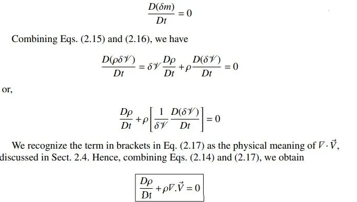
Equation (2.18) is the continuity equation in non-conservation form. In light of our philosophical discussion in Sect. 2.2, note that:
(1) By applying the model of an infinitesimal fluid element, we have obtained
Eq. (2.18) directly in partial differential form.
(2) By choosing the model to be moving with the flow, we have obtained the nonconservation form of the continuity equation, namely Eq. (2.18).
Now, consider the model of a finite control volume fixed in space, as sketched in Fig. 2.4. At a point on the control surface, the flow velocity is V vector and the vector elemental surface area (as defined in Sect. 2.4) is dS vector. Also let dV be an elemental volume inside the finite control volume. Applied to this control volume, our fundamental physical principle that mass is conserved means
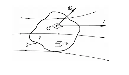
Finite control volume fixed in space
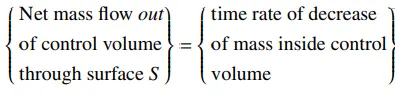
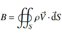
where B and C are just convenient symbols for the left and right sides, respectively, of Eq. (2.19a). First, let us obtain an expression for B in terms of the quantities shown in Fig. 2.4. The mass flow of a moving fluid across any fixed surface (say, in kg/s, or slug/s) is equal to the product of (density) × (area of surface) × (component of velocity perpendicular to the surface). Hence the elemental mass flow across the area dS is
ρVndS = ρV · dS (2.20)
Examining Fig. 2.4, note that by convention, dS always points in a direction out of the control volume. Hence, when V also points out of the control volume (as shown in Fig. 2.4), the product ρV · dS is positive. Moreover, when V points out of the control volume, the mass flow is physically leaving the control volume, i.e. it is an outflow. Hence, a positive ρV· dS denotes an outflow. In turn, when V points into the control volume, ρV ·dS is negative. Moreover, when V points inward, the mass flow is physically entering the control volume, i.e. it is an inflow. Hence, a negative ρV ·dS denotes an inflow. The net mass flow out of the entire control volume through the control surface S is the summation over S of the elemental mass flows shown in Eq. (2.20). In the limit, this becomes a surface integral, which is physically the left side of Eqs. (2.19a and b), i.e.
Now consider the right side of Eqs. (2.19a and b). The mass contained within the elemental volume dV is ρ dV. The total mass inside the control volume is therefore
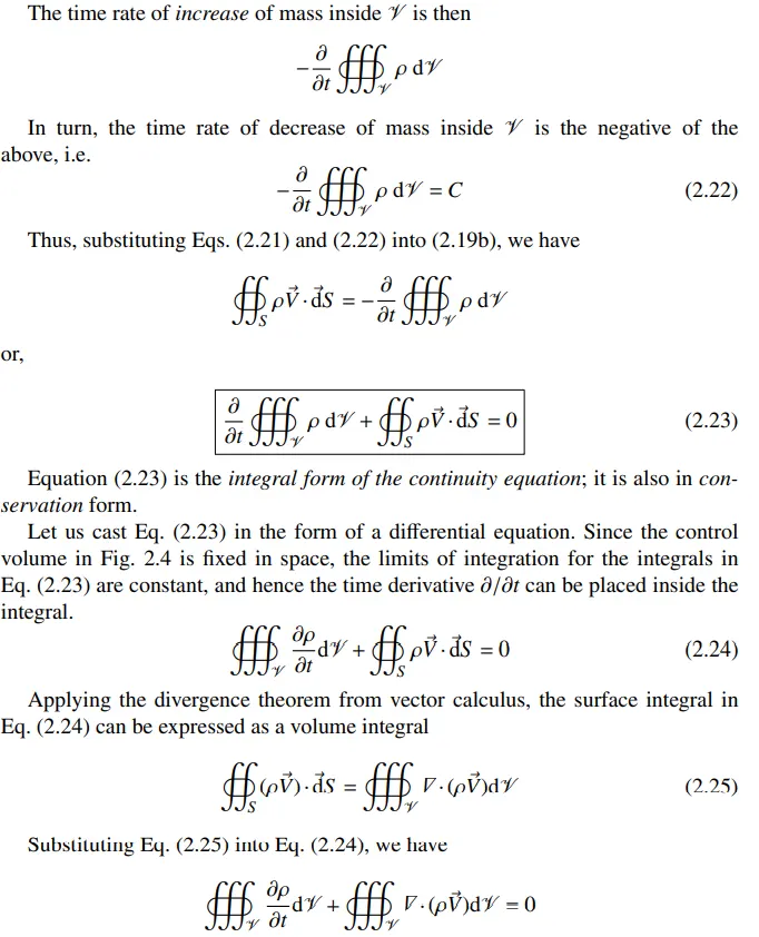
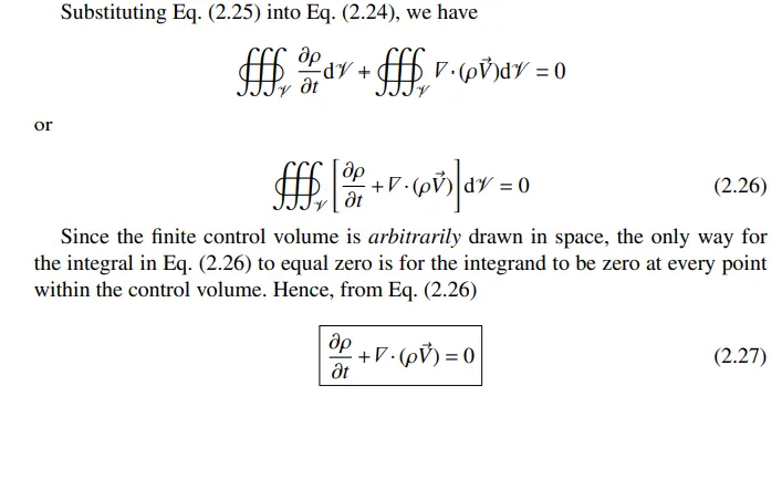
Momentum Equation
In this section, we apply another fundamental physical principle to a model of the flow, namely:
Physical Principle: F = ma (Newton’s 2nd law)
We choose for our flow model the moving fluid element as shown at the right of Fig. 2.1(b). This model is sketched in more detail in Fig. 2.5. Newton’s 2nd law, expressed above, when applied to the moving fluid element in Fig. 2.5, says that the net force on the fluid element equals its mass times the acceleration of the element. This is a vector relation, and hence can be split into three scalar relations along the x, y, and z-axes.
Let us consider only the x-component of Newton’s 2nd law,
Fx = max
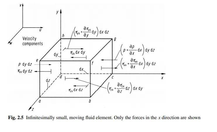
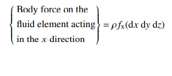
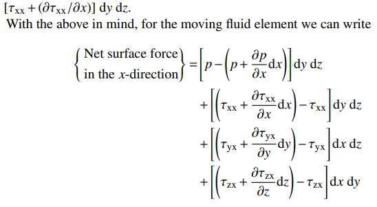
The total force in the x-direction, Fx, is given by the sum of Eqs. (2.31) and (2.32). Adding, and canceling terms, we obtain

Equation (2.33) represents the left-hand side of Eq. (2.30). Considering the right-hand side of Eq. (2.30), recall that the mass of the fluid
element is fixed and is equal to
m = ρ dx dy dz
Also, recall that the acceleration of the fluid element is the time rate-of-change of its velocity. Hence, the component of acceleration in the x-direction, denoted by ax, is simply the time-rate-of-change of u; since we are following a moving fluid element, this time-rate-of-change is given by the substantial derivative. Thus,
ax = Du/Dt, Combining Eqs. (2.30), (2.33), (2.34) and (2.35), we obtain
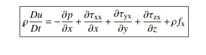
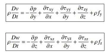
which is the x-component of the momentum equation for a viscous flow. In a similar fashion, the y and z components can be obtained as
The Navier–Stokes equations can be obtained in conservation form as follows. Writing the left-hand side of Eq. (2.36a) in terms of the definition of the substantial derivative,
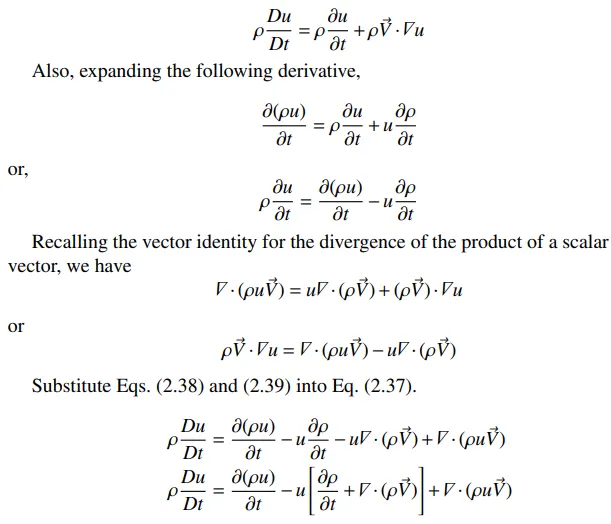
The term in brackets in Eq. (2.40) is simply the left-hand side of the continuity equation given as Eq. (2.27); hence the term in brackets is zero. Thus Eq. (2.40) reduces to
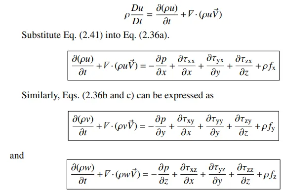
Equations (2.42a–c) are the Navier-Stokes equations in conservation form. In the late seventeenth century Isaac Newton stated that shear stress in a fluid is proportional to the time-rate-of-strain, i.e. velocity gradients. Such fluids are called Newtonian fluids. (Fluids in which τ is not proportional to the velocity gradients are non-Newtonian fluids; blood flow is one example.) In virtually all practical aerodynamic problems, the fluid can be assumed to be Newtonian. For such fluids, Stokes, in 1845, obtained:
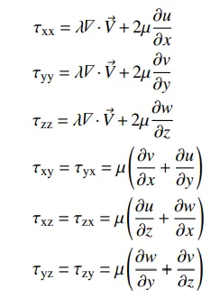
where μ is the molecular viscosity coefficient and λ is the bulk viscosity coefficient. Stokes made the hypothesis that
λ = −2/3 μ
which is frequently used but which has still not been definitely confirmed to the present day. 2 equations in conservation form: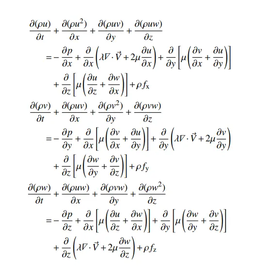
The Energy Equation
In the present section, we derive the energy equation using as our model an infinitesimal moving fluid element. This will be in keeping with our derivation of the Navier–Stokes equations in Sect. 2.6, where the infinitesimal element was shown in Fig. 2.5.
We now invoke the following fundamental physical principle:
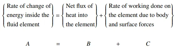
where A, B, and C denote the respective terms above. Let us first evaluate C, i.e. obtain an expression for the rate of work done on the
moving fluid element due to body and surface forces. It can be shown that the rate of doing work by a force exerted on a moving body is equal to the product of the force and the component of velocity in the direction of the force (see References 3 and 14 for such a derivation). Hence the rate of work done by the body force acting on the fluid element moving at a velocity V is
ρ f·V (dx dy dz)
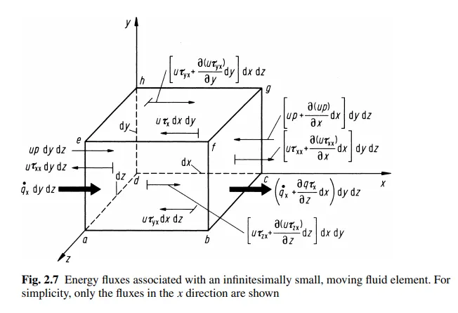
With regard to the surface forces (pressure plus shear and normal stresses), consider just the forces in the x-direction, shown in Fig. 2.5. The rate of work done on the moving fluid element by the pressure and shear forces in the x-direction shown in Fig. 2.5 is simply the x-component of velocity, u, multiplied by the forces, e.g. on the face and the rate of work done by τyxdx dz is uτyxdx dz, with similar expressions for the other faces. To emphasize these energy considerations, the moving fluid element is redrawn in Fig. 2.7, where the rate of work done on each face by surface forces in the x-direction is shown explicitly. To obtain the net rate of work done on the fluid element by the surface forces, note that forces in the positive x-direction do positive work and that forces in the negative x-direction do negative work. Hence,
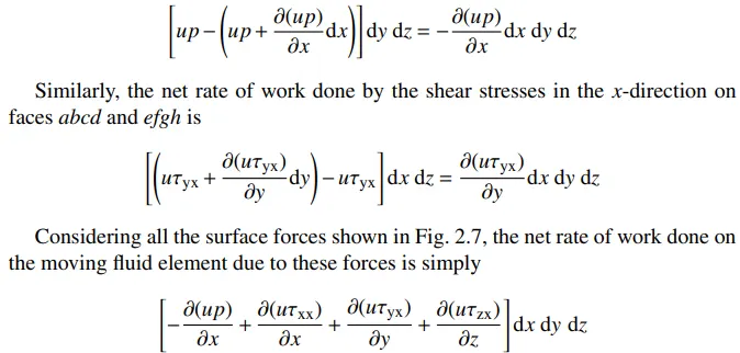
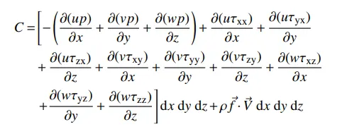
The above expression considers only surface forces in the x-direction. When the surface forces in the y- and z-directions are also included, similar expressions are obtained. In total, the net rate of work done on the moving fluid element is the sum of the surface force contributions in the x-, y- and z-directions, as well as the body force contribution. This is denoted by C in Eq. (2.45) and is given by
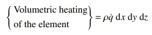
Let us turn our attention to B in Eq. (2.45), i.e. the net flux of heat into the element. This heat flux is due to: (1) volumetric heating such as absorption or emission of radiation, and (2) heat transfer across the surface due to temperature gradients, i.e. thermal conduction. Define ˙q as the rate of volumetric heat addition per unit mass. Noting that the mass of the moving fluid element in Fig. 2.7 is ρ dx dy dz, we obtain
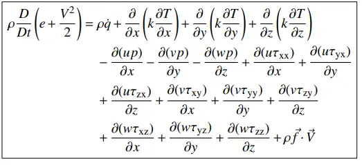
This is the non-conservation form of the energy equation; also note that it is in terms of the total energy, (e+V2/2). Once again, the non-conservation form results from the application of the fundamental physical principle to a moving fluid element. The left-hand side of Eq. (2.52) involves the total energy, (e+V2/2). Frequently, the energy equation is written in a form that involves just the internal energy, e. The derivation is as follows. Multiply Eqs. (2.36a, b, and c) by u, v, and w respectively.
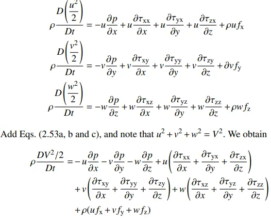
Add Eqs. (2.53a, b and c), and note that u2 +v2 +w2 = V2. We obtain
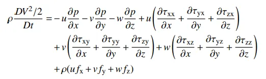
Subtracting Eq from Eq.noting that ρ f · V = ρ(u fx + v fy + w fz), we have
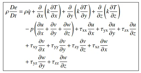
Equation (2.55) is the energy equation in terms of internal energy, e. Note that the body force terms have canceled; the energy equation when written in terms of e does not explicitly contain the body force. Eq. (2.55) is still in nonconservation form. Equations (2.52) and (2.55) can be expressed totally in terms of flow field variables by replacing the viscous stress terms τxy, τxz, etc. with their equivalent expressions from Eqs (2.43a, b, c, d, e, and f ). For example, from Eq. (2.55), noting that τxy = τyx, τxz = τzx, τyz = τzy,
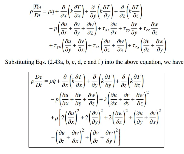
equation (2.56) is a form of the energy equation completely in terms of the flowfield variables. A similar substitution of Eqs. (2.43a, b, c, d, e and f ) can be made into Eq. (2.52); the resulting form of the energy equation in terms of the flow-field variables is lengthy, and to save time and space it will not be given here. The energy equation in conservation form can be obtained as follows. Consider the left-hand side of Eq. (2.56). From the definition of the substantial derivative:
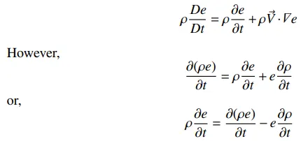
From the vector identity concerning the divergence of the product of scalar times a vector,
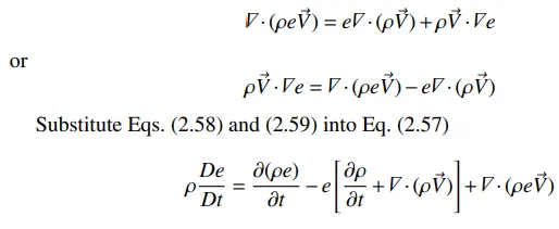
The term in square brackets in Eq. (2.60) is zero, from the continuity equation, Eq. (2.27). Thus, Eq. (2.60) becomes
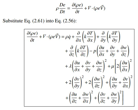
Equation (2.62) is the conservation form of the energy equation, written in terms of internal energy. Repeating the steps from Eq. (2.57) to Eq. (2.61), except operating on the total energy, (e+V2/2), instead of just the internal energy, e, we obtain
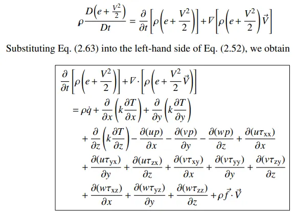
Equation (2.64) is the conservation form of the energy equation, written in terms of the total energy, (e+V2/2). As a final note in this section, there are many other possible forms of the energy equation; for example, the equation can be written in terms of enthalpy, h, or total enthalpy, (h + V2/2). We will not take the time to derive these forms here; see Refs. [1–3] for more details.
Summary of the Governing Equations for Fluid Dynamics: With Comments
By this point in our discussions, you have seen a large number of equations, and they may seem to you at this stage to be ‘all looking alike’. Equations by themselves can be tiring, and this chapter would seem to be ‘wall-to-wall’ equations. However, all of theoretical and computational fluid dynamics is based on these equations, and therefore it is absolutely essential that you are familiar with them, and that you understand their physical significance. That is why we have spent so much time and effort in deriving the governing equations. Considering this time and effort, it is important to now summarize the important forms of these equations, and to sit back and digest them.
PHYSICAL PROBLEM: SUBSONIC-SUPERSONIC ISENTROPIC FLOW
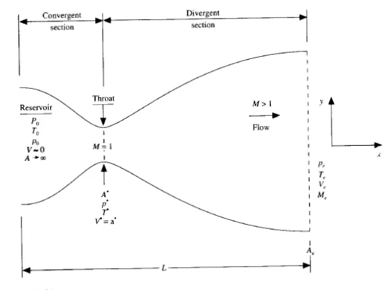
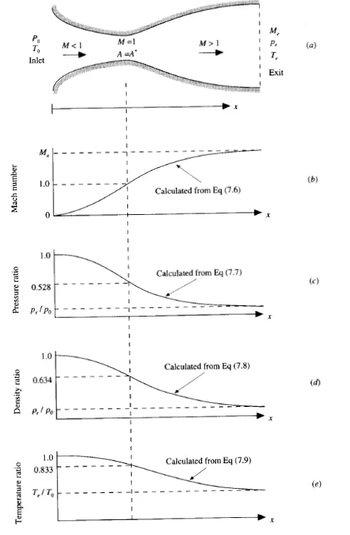
We consider the steady, isentropic flow through a convergent-divergent nozzl_e as sketched in Fig. 7 .1. The flow at the inlet to the nozzle comes from a_ reservoir where the pressure and temperature are denoted by p0 , and To, respectively. The cross-sectional area of the reservoir is large ( theoretically, A --+ oo ), and hence the velocity is very small ( V --+ O). Thus, Po and T0 are the stagnatio~ values,_ or total pressure and total temperature, r~spectively. Th~ flow expands 1sentrop1cally. to supersonic speeds at the nozzle exit, where the exit pressure, temperature, veloc11?", and Mach number are denoted by Pe, Te, V.,, and Me, respectlv~ly. The flow IS locally subsonic in the convergent section ?f the nozzl~, some at th~ throat (minimum area), and supersonic at the d1ver~ent sec~1on. T?e ~omc flow (M = 1) at the throat means that the local velocity at this location 1s equal to the local speed of sound.
Using an asterisk to denote sonic flow values, we have at the throat V = V* = a*. Similarly, the sonic flow values of pressure and temperature are denoted by p* and T*, respectively. The area of the sonic throat is denoted by A*. We assume that at a given section, where the cross-sectional area is A, the flow properties are uniform across that section. Hence, although the area of the nozzle changes as a function of distance along the nozzle, x, and therefore in reality the flow field is two-dimensional (the flow varies in.the two-dimensional .ry space), we make the assumption that the flow properties-vary only with x; this is tantamount to assuming uniform flow properties across any given cross section. Such flow is defined as quasi-one-dimensional flow.
SUBSONICSUPERSONIC ISENTROPIC NOZZLE FLOW· MACCORMACK'S TECHNIQUE
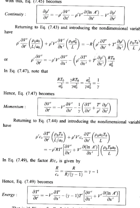
We are finally finished with the first echelon as itemized at the beg~nning of this subsection. After what may seem like an interminable manipulation of the governing equations, we have finally set up that particular form of the equations that will be most appropriate as well as convenient for the time-marching solution of quasi-one-dimensional nozzle flow. which is exactly represented in John Andersons book of CFD.
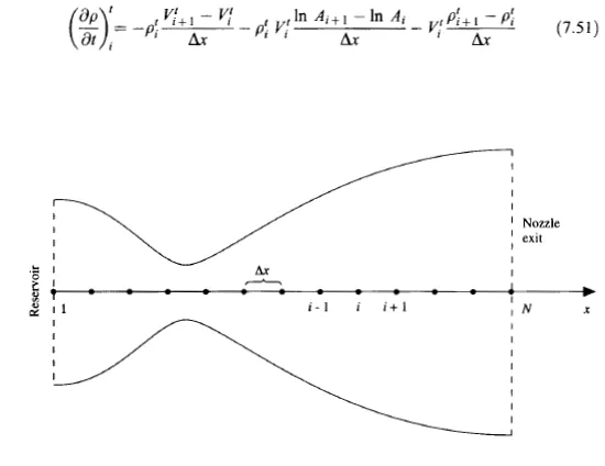
The same approach is taken for the MATLAB coding where we run programming of conservation and nonconservation equations with Mccormack's method. We made a function of both and the calling it in main program.
Function of Non-Conservation form
function [mfr,v,t,p,rho,m_throat,p_throat,t_throat,rho_throat,x]= non_conservative(n,nt)


x=linspace(0,3,n);   %meshing the domain
dx=x(2)-x(1);        %element size
gama=1.4;            %gamma value
throat=(n+1)/2;      %node number of the throat


%intial conditions
rho=1-0.3146.*x;
t=1-0.2314.*x;
v=(0.1+1.09*x).*t.^0.5;


%area
a=1+2.2*(x-1.5).^2;


%time steps & time step size calulation based on courant number
w=nt;
c=0.5;
dt=min(c.*dx./(sqrt(t)+v));


for k=1:w     %time loop

    rho_old=rho;
    v_old=v;
    t_old=t;   %saving the intial values


    %predictor step
    for j =2:n-1

        %drho_dt_p=-rho(j)*(v(j+1)-v(j))/dx-rho(j)*v(j)*((log(a(j+1))-log (a(j)))/dx)-v(j)*((rho(j+1)-rho(j))/dx);
        dvdx=(v(j+1)-v(j))/dx;
        drhodx=((rho(j+1)-rho(j))/dx);
        dtdx=(t(j+1)-t(j))/dx;
        dlogadx=(log(a(j+1))-log(a(j)))/dx;

                                                                    %continuity equations in non conservative form
        drhodt_p(j)=-rho(j)*dvdx-rho(j)*v(j)*dlogadx-v(j)*drhodx;
                                                                     % momentum equations in non conservative form
        dvdt_p(j)=-v(j)*dvdx-(1/gama)*(dtdx+(t(j)/rho(j))*drhodx);
                                                                      %energy equations in non conservative form
        dtdt_p(j)=-v(j)*dtdx-(gama-1)*t(j)*(dvdx+v(j)*dlogadx);

        rho(j)=rho(j)+drhodt_p(j)*dt;               %solution update after prdictor step
        v(j)=v(j)+dvdt_p(j)*dt;
        t(j)=t(j)+dtdt_p(j)*dt;
    end


    %corrector step
    for j =2:n-1
        %drho_dt_p=-rho(j)*(v(j+1)-v(j))/dx-rho(j)*v(j)*((log(a(j+1))-log (a(j)))/dx)-v(j)*((rho(j+1)-rho(j))/dx);
        dvdx=(v(j)-v(j-1))/dx;
        drhodx=((rho(j)-rho(j-1))/dx);
        dtdx=(t(j)-t(j-1))/dx;
        dlogadx=(log(a(j))-log(a(j-1)))/dx;

        drhodt_c(j)=-rho(j)*dvdx-rho(j)*v(j)*dlogadx-v(j)*drhodx;

        dvdt_c(j)=-v(j)*dvdx-(1/gama)*(dtdx+(t(j)/rho(j))*drhodx);

        dtdt_c(j)=-v(j)*dtdx-(gama-1)*t(j)*(dvdx+v(j)*dlogadx);
    end


    %average time derivative
    drhodt=0.5*(drhodt_p+drhodt_c);
    dvdt=0.5*(dvdt_p+dvdt_c);
    dtdt=0.5*(dtdt_p+dtdt_c);


    %final solution update
    for i=2:n-1
    rho(i)=rho_old(i)+drhodt(i)*dt;
    v(i)=v_old(i)+dvdt(i)*dt;
    t(i)=t_old(i)+dtdt(i)*dt;
    end


    %bc inlet
    v(1)=2*v(2)-v(3);

    %outlet
    v(n)=2*v(n-1)-v(n-2);
    rho(n)=2*rho(n-1)-rho(n-2);
    t(n)=2*t(n-1)-t(n-2);


    %pressure
    p=rho.*t;
    %mach number
    m=v./(t.^0.5);
    %mass flow rate
    mfr=rho.*v.*a;


    if k==10
        figure(1) %mass flow rate @ different time steps vs (analytical) mass flow rate
        plot(x,mfr,'r')
        hold on
    elseif k==300
        figure(1)
        plot(x,mfr,'g')
        hold on
    elseif k==500
        figure(1)
        plot(x,mfr,'b')
        hold on
    elseif k==700
        figure(1)
        plot(x,mfr,'k')
        xlabel('x/L')
        ylabel('Mass Flow Rate')
        title('Mass flow rate at various time steps -Non-Conservative form')
        hold on
        line([0 3],[0.579 0.579],'Color','m','Marker','d','Markersize',10) %analytical mass flow rate = 0.579
        legend('10dt','300dt','500dt','700dt','Analytical','Location','Northeast')
        hold on
    end

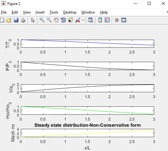
    figure(2)%steady state distribution
    subplot(5,1,1)
    plot(x,t,'b')
    ylabel('T/T_{0}')


    subplot(5,1,2)
    plot(x,p,'k')
    ylabel('P/P_{0}')

    subplot(5,1,3)
    plot(x,v,'k')
    ylabel('V/a_{0}')

    subplot(5,1,4)
    plot(x,rho,'g')
    ylabel('rho/rho_{0}')

    subplot(5,1,5)
    plot(x,m,'y')
    ylabel('Mach no')
    xlabel('x/L')
    title('Steady state distribution-Non-Conservative form')

    %saving the throat values of primitive variables for different time
    %steps
    t_throat(k)=t(throat);
    p_throat(k)=p(throat);
    rho_throat(k)=rho(throat);
    m_throat(k)=m(throat);

    figure(3)%time variation @ throat
    subplot(4,1,1)
    plot(t_throat,'k')
    ylabel('T/T_{0}')

    subplot(4,1,2)
    plot(p_throat,'k')
    ylabel('P/P_{0}')

    subplot(4,1,3)
    plot(rho_throat,'k')
    ylabel('rho/rho_{0}')

    subplot(4,1,4)
    plot(m_throat,'k')
    ylabel('Mach no')
    xlabel('No of time steps')
    title('Time variation-Non-Conservative form')

end
end
Function of Conservation-Form
function [mfr,v,t,p,rho,m_throat,p_throat,t_throat,rho_throat]= conservative(n,nt)


x=linspace(0,3,n); %meshing the domain
dx=x(2)-x(1); %element size
gama=1.4; %gamma value
throat=(n+1)/2;  %node number of the throat

a=1+2.2*(x-1.5).^2;

for i=1:length(x)               %intial conditions
    if x(i)>= 0 && x(i)<= 0.5
        rho(i)=1;
        t(i)=1;
    elseif x(i)>=0.5 && x(i)<=1.5
        rho(i)=1-0.366*(x(i)-0.5);
        t(i)=1-0.167*(x(i)-0.5);
    elseif x(i)>=1.5 && x(i)<= 3.0
        rho(i)=0.634-0.3879*(x(i)-1.5);
        t(i)=0.833-0.3507*(x(i)-1.5);
    end
end


v=0.59./(rho.*a);  %calcualting v & rho from the fixed intial conditions
p=rho.*t;

%initial solution vectors
u1=rho.*a;
u2=rho.*a.*v;
u3=rho.*a.*(t./(gama-1)+(gama/2).*v.^2);

%time steps & time step size calulation based on courant number
w=nt;
c=0.5;
dt=min(c.*dx./(sqrt(t)+v));

for k=1:w    %time loop

    u1_old=u1;
    u2_old=u2;
    u3_old=u3;    %saving the intial values

    f1=u2;         %flux vectors calculated from the initial solution vector
    f2=(u2.^2./u1)+((gama-1)/(gama)*(u3-(gama*u2.^2)./(2*u1)));
    f3=((gama*u2.*u3)./u1)-((gama*(gama-1))/2)*((u2.^3)./(u1.^2));

    %predictor step
    for j=2:n-1

        %source term
        j2(j)=(1/gama)*rho(j)*t(j)*((a(j+1)-a(j))/dx);

        df1dx=(f1(j+1)-f1(j))/dx;
        df2dx=(f2(j+1)-f2(j))/dx;
        df3dx=(f3(j+1)-f3(j))/dx;


        du1dt_p(j)=-df1dx;  %continuity equations in conservative form
        du2dt_p(j)=-df2dx+j2(j);   % momentum equations in conservative form
        du3dt_p(j)=-df3dx;  %energy equations in conservative form

        u1(j)=u1(j)+du1dt_p(j)*dt;    %solution vectors are updated after prdictor step
        u2(j)=u2(j)+du2dt_p(j)*dt;
        u3(j)=u3(j)+du3dt_p(j)*dt;
    end

    rho=u1./a;                              %calculting primitive variables from the predictor solution vectors
    v=u2./u1;
    t=(gama-1)*(u3./u1-(gama/2)*v.^2);
    p=rho.*t;

    f1=u2;                                %updating flux vectors from the predictor solution vectors
    f2=((u2.^2)./u1)+((gama-1)/gama)*(u3-((gama*u2.^2)./(2*u1)));
    f3=(gama*u2.*u3./u1)-(gama*(gama-1)/2)*(u2.^3./u1.^2);

    %corrector step
    for j=2:n-1

        %source term
        j2(j)=(1/gama)*rho(j)*t(j)*((a(j)-a(j-1))/dx);

        df1dx=(f1(j)-f1(j-1))/dx;
        df2dx=(f2(j)-f2(j-1))/dx;
        df3dx=(f3(j)-f3(j-1))/dx;


        du1dt_c(j)=-df1dx;
        du2dt_c(j)=-df2dx+j2(j);
        du3dt_c(j)=-df3dx;

    end

        %average time derivative
        du1dt=0.5*(du1dt_p+du1dt_c);
        du2dt=0.5*(du2dt_p+du2dt_c);
        du3dt=0.5*(du3dt_p+du3dt_c);

        for m=2:n-1 %final solution update
        u1(m)=u1_old(m)+du1dt(m)*dt;
        u2(m)=u2_old(m)+du2dt(m)*dt;
        u3(m)=u3_old(m)+du3dt(m)*dt;
        end


        %bc @ inlet
        u1(1)=rho(1).*a(1);
        u2(1)=(2*u2(2))-u2(3);
        u3(1)=u1(1)*(t(1)/(gama-1)+(gama/2)*v(1).^2);

        %bc @ outlet
        u1(n)=2*u1(n-1)-u1(n-2);
        u2(n)=2*u2(n-1)-u2(n-2);
        u3(n)=2*u3(n-1)-u3(n-2);


    rho=u1./a;          %extracting primitive variables from the solution vectors
    v=u2./u1;
    t=(gama-1)*((u3./u1)-(gama/2)*v.^2);
    p=rho.*t;


    %mach no calculation
    m=(v)./(t.^0.5);
    mfr=rho.*v.*a; %mass flow rate calculation


    if k==100              %mass flow rate @ different time steps vs mass flow rate (analytical)
        figure(4)
        plot(x,mfr,'r')
        hold on
    elseif k==300
        figure(4)
        plot(x,mfr,'g')
        hold on
    elseif k==500
        figure(4)
        plot(x,mfr,'b')
        hold on
    elseif k==700
        figure(4)
        plot(x,mfr,'k')
        xlabel('x')
        ylabel('mass flow rate')
        title('Mass flow rate at various time steps Conservative form')
        hold on
        line([0 3],[0.579 0.579],'Color','m','Marker','d','Markersize',10)    %analytical mass flow rate = 0.579
        legend('100dt','300dt','500dt','700dt','Analytical','Location','Northeast')
        hold on
    end


    figure(5)             %steady state distribution
    subplot(5,1,1)
    plot(x,t,'b')
    ylabel('T/T_{0}')


    subplot(5,1,2)
    plot(x,p,'k')
    ylabel('P/P_{0}')

    subplot(5,1,3)
    plot(x,v,'k')
    ylabel('V/a_{0}')

    subplot(5,1,4)
    plot(x,rho,'g')
    ylabel('rho/rho_{0}')

    subplot(5,1,5)
    plot(x,m,'y')
    ylabel('Mach no')
    xlabel('x/L')
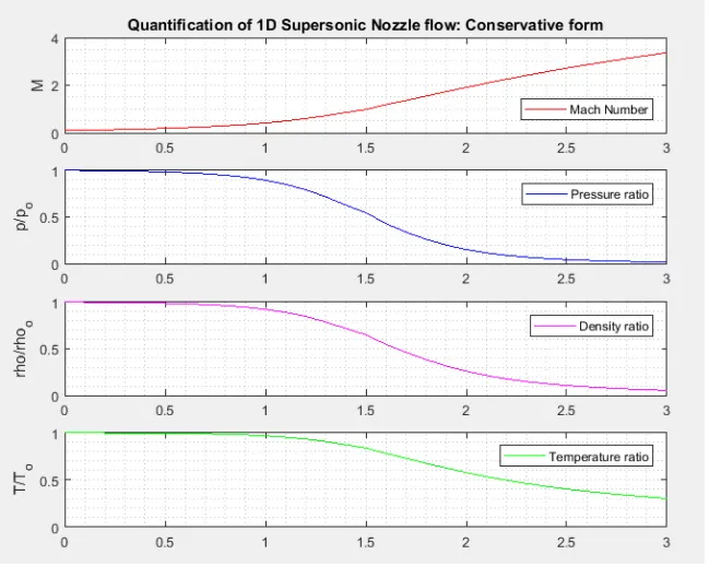
    title('Steady state distribution-Conservative form')

    %saving the throat values of primitive variables for different time
    %steps
    t_throat(k)=t(throat);
    p_throat(k)=p(throat);
    rho_throat(k)=rho(throat);
    m_throat(k)=m(throat);


    figure(6)                  %time variation @ throat
    subplot(4,1,1)
    plot(t_throat,'k')
    ylabel('T/T_{0}')

    subplot(4,1,2)
    plot(p_throat,'k')
    ylabel('P/P_{0}')

    subplot(4,1,3)
    plot(rho_throat,'k')
    ylabel('rho/rho_{0}')

    subplot(4,1,4)
    plot(m_throat,'k')
    ylabel('Mach no')
    xlabel('No of time steps')
    title('Time variation-Conservative form')

end
end
Main Program:
clear all
close all
clc

n=61;  %no of grid points
nt=1400; %number of time steps

%calling Conservative function
[mfr_NON_consv,v,t,p,rho,m_throat,p_throat,t_throat,rho_throat,x]=non_conservative(n,nt);

%calling Non-Conservative function
[mfr_consv,v_consv,t_consv,p_consv,rho_consv,m_throat_c,p_throat_C,t_throat_C,rho_throat_C]=conservative(n,nt);

%comparing mass flow rate of conservative, non conservative & analytical
%forms
figure(7)
plot(x,mfr_NON_consv,'r')
hold on
plot(x,mfr_consv,'b')
hold on
line([0 3],[0.579 0.579],'Color','k','Marker','d','Markersize',10)    %analytical mass flow rate = 0.579
hold on
xlabel('x/L')
ylabel('Mass flow rate')
legend('Non Conservative','Conservative','Analytical')
Output:
1. Spatial details on Density, Pressure, Mach no. Temperature fields at n = 61.
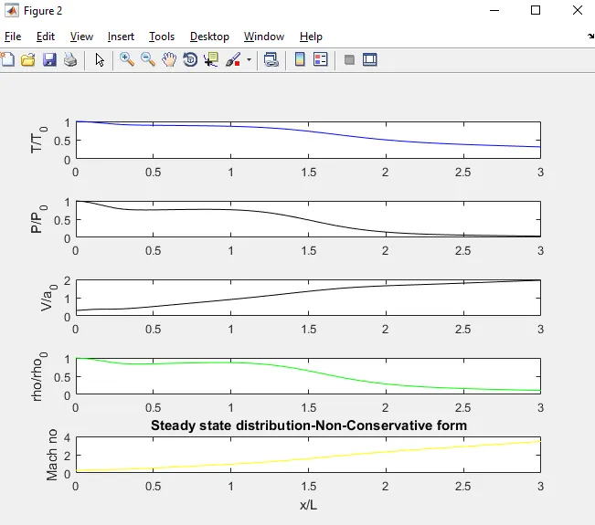
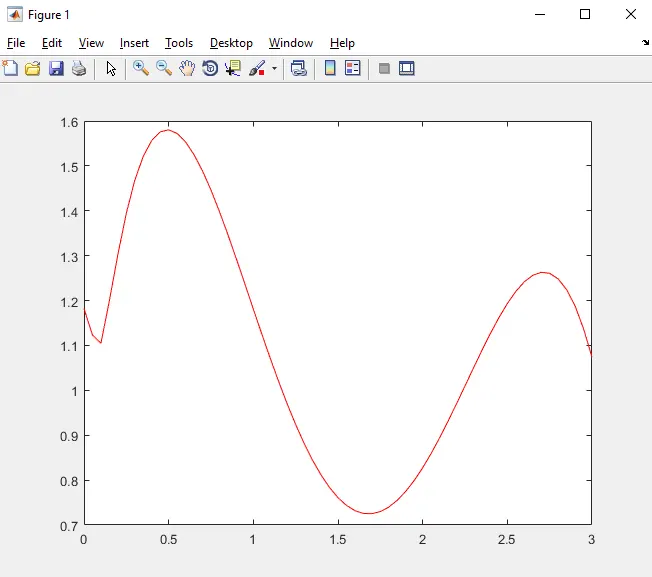
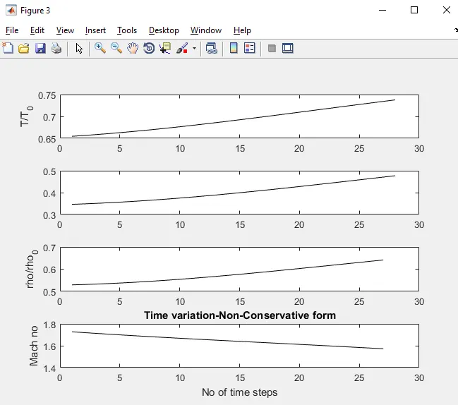
3. Spatial details on Density, Pressure, Mach no. Temperature fields at n = 31.
Conclusion:
The Conservative converges faster than the nonconservative form with less computational time as it attains the quicker solution at the initial stage.
References:
fluidsreview-1.pdf (auburn.edu)
John Anderson's CFD book