Week 7 - Simulation of a 1D Super-sonic nozzle flow simulation using Macormack Method
Abstract: In this study, conservative and non-conservative forms of governing equations to solve quasi 1D isentropic nozzle flow using MacCormak technique. Here we compare the results to evident their differences.
Introduction:
Conservation governing flow equations:
1. Continuity:
`(delrho')/(delt')=-rho'(delV')/(delx')-rho'V'(del(lnA'))/(delx')-V'(delrho')/(delx')`
2. Momentum:
`(delV')/(delt')=-V'(delV')/(delx')-1/gamma((delT')/(delx')+(T')/(rho')(delrho')/(delx'))`
3. Energy:
`(delT')/(delt')=-V'(delT')/(delx')-(1-gamma)T'[(delV')/(delx')+V'((del(lnA'))/(delx'))]`
Non Conservation governing flow equations:
1. Continuity:
`(del(rho'A'))/(delt')+(del(rho'A'V'))/(delx')=0`
where
`U1=rho'A'`
`F1=rho'A'V'`
2. Momentum:
`(del(rho'A'V'))/(delt')+(del(rho'A'V'overset(2)()+(1/gamma)p'A'))/(delx')=(1/gamma)p'(delA')/(delx')`
where
`U2=rho'A'V'`
`F2=(del(rho'A'V'overset(2)()+(1/gamma)p'A'))/(delx')`
`J1=(1/gamma)p'(delA')/(delx')`
3. Energy:
`(del[rho'((e')/(gamma-1)+gamma/2V'overset(2)())A'])/(delt')+(del[rho'((e')/(gamma-1)+gamma/2V'overset(2)()]V'A'+p'A'V')]/(delx')=0`
where
`U3=rho'((e')/(gamma-1)+gamma/2V'overset(2)())A'`
`F3=rho'((e')/(gamma-1)+gamma/2V'overset(2)())V'A'+p'A'V'`
Maccormack's Technique:
MacCormack method is an explicit finite-difference technique which is second order accurate in both space and time.
Step 1: Predictor Step - Utilize forward differences for the right-hand side spatial derivatives.
Step 2: Corrector step - By primitive variables with respect to predicted values from 'Step 1' and by applying backward differences to the updated right-hand side spatial derivatives.
Step 3: Average of the derivatives from predictor and corrector step is calculated.
Step 4: Updating the primitive variables for all the grid points for the respective time step with respect to average derivative calculated using 'step 3'
Now the above steps will be repeated for a respective number of time steps.
Main Program
% % Simulation of a 1D Super-sonic nozzle flow simulation using Macormack Method
clear all
close all
clc
%% Inputs
n=31;
x=linspace(0,3,n)
dx=x(2)-x(1)
gamma = 1.4;
c=0.5;
% Area
% Time steps
nt = 1400,
tic
[rho_c,pr_c,t_c,v_c,mach_c,mfr_c,rho_th_c,v_th_c,pr_th_c,mach_th_c,t_th_c,rho_exact,pr_exact,t_exact,mach_exact,mfr_exact,dU1dt_residual,dU2dt_residual,dU3dt_residual]=conservative_form(n,x,dx,gamma,c,nt)
time_counter=toc;
tic
[rho,pr,t,v,mach,mfr,rho_th_nc,v_th_nc,pr_th_nc,mach_th_nc,t_th_nc,rho_exact,pr_exact,t_exact,mach_exact,mfr_exact,drho_dt_residual,dv_dt_residual,dt_dt_residual]=non_conservation_form(n,x,dx,gamma,c,nt)
time_counter=toc;

figure(3)
subplot(4,1,1)
plot(rho_th_c,'linewidth',2)
hold on
plot(rho_th_nc,'linewidth',2)
plot(rho_exact,'linewidth',2)
xlabel('Time Step')
ylabel('rho/{rho_0}')
title('Variation of density, temperature, pressure & mach number at the nozzle throat using conservation form & non conservation form')
legend('Conservative form','Non onservative form','Exact solution')

subplot(4,1,2)
plot(t_th_c,'linewidth',2)
hold on
plot(t_th_nc,'linewidth',2)
plot(t_exact,'linewidth',2)
xlabel('Time Step')
ylabel('t/{t_0}')
legend('Conservative form','Non onservative form','Exact solution')

subplot(4,1,3)
plot(pr_th_c,'linewidth',2)
hold on
plot(pr_th_nc,'linewidth',2)
plot(pr_exact,'linewidth',2)
xlabel('Time Step')
ylabel('p/{p_0}')
legend('Conservative form','Non onservative form','Exact solution')

subplot(4,1,4)
plot(mach_th_c,'linewidth',2)
hold on
plot(mach_th_nc,'linewidth',2)
plot(mach_exact,'linewidth',2)
xlabel('Time Step')
ylabel('mach no')
legend('Conservative form','Non onservative form','Exact solution')

mfr_exact = 0.579;
figure(4)
plot(x,mfr_c)
hold on
plot(x,mfr)
plot(x,mfr_exact,'k')
hold off
xlabel('Nozzle length')
ylabel('mass flow rate')
title(' Comparison of Mass flow rate using conservation form & non conservation form w.r.t exact value')
legend('Conservative','Non conservative','Exact')


figure(5)
subplot(4,1,1)
plot(rho_c)
hold on
plot(rho)
xlabel('Nozzle length')
ylabel('Density')
title('Variation of density, temperature, pressure & mach number along the nozzle length using conservation form & non conservation form')
legend('Conservative','Non conservative')

subplot(4,1,2)
plot(t_c)
hold on
plot(t)
xlabel('Nozzle length')
ylabel('Temperature')
legend('Conservative','Non conservative')

subplot(4,1,3)
plot(pr_c)
hold on
plot(pr)
xlabel('Nozzle length')
ylabel('Pressure')
legend('Conservative','Non conservative')

subplot(4,1,4)
plot(mach_c)
hold on
plot(mach)
xlabel('Nozzle length')
ylabel('Mach no')
legend('Conservative','Non conservative')


figure(6)
subplot(2,1,1)
semilogy(drho_dt_residual)
hold on
semilogy(dv_dt_residual)
semilogy(dt_dt_residual)
xlabel('Residual')
ylabel('Time step')
title('Residual of density, temperature, pressure & mach number results by using non conservation form')
legend('Density','Velocity','Temperature')

subplot(2,1,2)
semilogy(dU1dt_residual)
hold on
semilogy(dU2dt_residual)
semilogy(dU3dt_residual)
xlabel('Residual')
ylabel('Time step')
title('Residual of solution vectors results by using conservation form')
legend('dU1dt residual','dU2dt residual','dU3dt residual')
Conservation function program
function[rho_c,pr_c,t_c,v_c,mach_c,mfr_c,rho_th_c,v_th_c,pr_th_c,mach_th_c,t_th_c,rho_exact,pr_exact,t_exact,mach_exact,mfr_exact,dU1dt_residual,dU2dt_residual,dU3dt_residual]=conservative_form(n,x,dx,gamma,c,nt)
%Area
a=1+2.2*(x-1.5).^2;
%Throat area
th=find(a==1)
%Initial condition
for i=1:n
 if(x(i)>=0 && x(i)<=0.5)
    rho_c(i)=1;
    t_c(i)=1;
 elseif (x(i)>=0.5 && x(i)<=1.5)
    rho_c(i)=1-0.366*(x(i)-0.5);
    t_c(i)=1-0.167*(x(i)-0.5);
 elseif (x(i)>=1.5 && x(i)<=3.5)
    rho_c(i)=0.634-0.3879*(x(i)-1.5);
    t_c(i)=0.833-0.3507*(x(i)-1.5);
 end
end
v_c=0.59./(rho_c.*a);

pr=rho_c.*t_c;
U1=rho_c.*a;
U2=rho_c.*a.*v_c;
U3=U1.*((t_c./(gamma-1))+((gamma/2).*(v_c.^2)));

for k=1:nt
  dt=min(c.*(dx./((t_c.^0.5)+v_c)));
  U1_old=U1;
  U2_old=U2;
  U3_old=U3;

  F1=U2;
  F2=((U2.^2)./U1)+(((gamma-1)/gamma)*(U3-((gamma/2)*((U2.^2)./U1))));
  F3=((gamma*U2.*U3)./U1)-(gamma*(gamma-1)*(U2.^3))./(2*U1.^2);
% Step 1: Predictor step
for i=2:n-1

  dF1dx(i)=(F1(i+1)-F1(i))/dx;
  dF2dx(i)=(F2(i+1)-F2(i))/dx;
  dF3dx(i)=(F3(i+1)-F3(i))/dx;

  dadx(i)=(a(i+1)-a(i))/dx;

  J2(i)=(1/gamma)*(rho_c(i)*t_c(i))*dadx(i);

  dU1dt_P(i)=-dF1dx(i);
  dU2dt_P(i)=-dF2dx(i)+J2(i);
  dU3dt_P(i)=-dF3dx(i);

  U1(i)=U1(i)+dU1dt_P(i)*dt;
  U2(i)=U2(i)+dU2dt_P(i)*dt;
  U3(i)=U3(i)+dU3dt_P(i)*dt;

end

rho_c=U1./a;
v_c=U2./U1;
t_c=(gamma-1)*((U3./U1)-((gamma*v_c.^2)/2));

F1=U2;
F2=((U2.^2)./U1)+(((gamma-1)/gamma)*(U3-((gamma/2)*((U2.^2)./U1))));
F3=((gamma*U2.*U3)./U1)-(gamma*(gamma-1)*(U2.^3))./(2*U1.^2);

%Step 2: Corrector step
for i=2:n-1

  dF1dx(i)=(F1(i)-F1(i-1))/dx;
  dF2dx(i)=(F2(i)-F2(i-1))/dx;
  dF3dx(i)=(F3(i)-F3(i-1))/dx;

  dadx1(i)=(a(i)-a(i-1))/dx;

  J3(i)=(1/gamma)*(rho_c(i)*t_c(i))*dadx1(i);

  dU1dt_C(i)=-dF1dx(i);
  dU2dt_C(i)=-dF2dx(i)+J3(i);
  dU3dt_C(i)=-dF3dx(i);

end

%Step 3
dU1dt=0.5*(dU1dt_P+dU1dt_C);
dU2dt=0.5*(dU2dt_P+dU2dt_C);
dU3dt=0.5*(dU3dt_P+dU3dt_C);
% Step 4
for j=2:n-1

  U1(j)=U1_old(j)+dU1dt(j)*dt;
  U2(j)=U2_old(j)+dU2dt(j)*dt;
  U3(j)=U3_old(j)+dU3dt(j)*dt;

end

U1(1)=a(1);
U2(1)=2*U2(2)-U2(3);
U3(1)=U1(1)*((t_c(1)/(gamma-1))+((gamma/2)*v_c(1)^2));

U1(n)=2*(U1(n-1))-U1(n-2);
U2(n)=2*(U2(n-1))-U2(n-2);
U3(n)=2*(U3(n-1))-U3(n-2);
  rho=U1./a;
  v=U2./U1;
  T=(gamma-1)*((U3./U1)-((gamma*v_c.^2)/2));
  mach_c= v_c./((t_c).^0.5);
  mfr_c=rho_c.*a.*v_c;
  pr_c=rho_c.*t_c;
  rho_th_c(k)=rho_c(th);
  v_th_c(k)=v_c(th);
  t_th_c(k)=t_c(th);
  pr_th_c(k)=pr_c(th);
  mach_th_c(k)=mach_c(th);
mfr_exact=0.579;
rho_exact=0.634*ones(1,1400);
t_exact=0.833*ones(1,1400);
pr_exact=0.528*ones(1,1400);
mach_exact=1*ones(1,1400);

dU1dt_residual(k)=abs(dU1dt(th));
dU2dt_residual(k)=abs(dU2dt(th));
dU3dt_residual(k)=abs(dU3dt(th));

% Plot for mass flow rate at random time steps
figure(1)
hold on
if (k==1)
    plot(x,mfr_c,'g','linewidth',2);
    else if (k==100)
     plot(x,mfr_c,'b','linewidth',2);
     else if (k==200)
      plot(x,mfr_c,'r','linewidth',2);
      else if (k==700)
      plot(x,mfr_c,'y','linewidth',2);
      legend('0dt','100dt','200dt','700dt')
      xlabel('x/L')
      ylabel('rhova/{rho_0v_0a_0}')
      title({'Variation of mass flow rate using conservation form at random time steps'})
      legend('1dt','100dt','200dt','700dt')
      grid minor
      end
     end
   end
  end
end
Non conservation function program
function[rho,pr,t,v,mach,mfr,rho_th_nc,v_th_nc,pr_th_nc,mach_th_nc,t_th_nc,rho_exact,pr_exact,t_exact,mach_exact,mfr_exact,drho_dt_residual,dv_dt_residual,dt_dt_residual]=non_conservation_form(n,x,dx,gamma,c,nt)
%Initial Condition
rho=1-0.3146*x;
t=1-0.2314*x;
v=(0.1+1.09*x).*t.^0.5;
a=1+2.2*(x-1.5).^2;
%Time Step Calculation
dt=min(c.*(dx./((t.^0.5+v))));
th=find(a==1);
for k=1:nt
 % dt=min(c.*(dx./((t.^0.5+v))));
  rho_old=rho;
    v_old=v;
    t_old=t;
    %Step 1: Predictor method
    %Continuity equation
    for j=2:n-1
    dvdx=(v(j+1)-v(j))/dx;
    drhodx=(rho(j+1)-rho(j))/dx;
    dtdx=(t(j+1)-t(j))/dx;
    dlogadx=(log(a(j+1))-log(a(j)))/dx;
    %Continuity Equation
    drho_dt_p(j)=-rho(j)*dvdx-rho(j)*v(j)*dlogadx-v(j)*drhodx;
    %Momentum Equation
    dv_dt_p(j)=-v(j)*dvdx-(1/gamma)*(dtdx+(t(j)/rho(j))*drhodx);
    %Energy Equation
    dt_dt_p(j)=-v(j)*dtdx-(gamma-1)*t(j)*(dvdx+v(j)*  dlogadx);
    %Solution step
    rho(j)=rho(j)+drho_dt_p(j)*dt;
    v(j)=v(j)+dv_dt_p(j)*dt;
    t(j)=t(j)+dt_dt_p(j)*dt;
  end
  %Step 2: Corrector Method
  for j=2:n-1
     %drho_dt_p=-rho(j)*(v(j+1)-v(j))/dx-rho(j)*v(j)*(log(a(j+1))-log(a(j)))/dx-v(j)*(rho(j+1)-rho(j))/dx;
    dvdx=(v(j)-v(j-1))/dx;
    drhodx=(rho(j)-rho(j-1))/dx;
    dtdx=(t(j)-t(j-1))/dx;
    dlogadx=(log(a(j))-log(a(j-1)))/dx;
    %Continuity Equation
    drho_dt_c(j)=-rho(j)*dvdx-rho(j)*v(j)*dlogadx-v(j)*drhodx;
    %Momentum Equation
    dv_dt_c(j)=-v(j)*dvdx-(1/gamma)*(dtdx+(t(j)/rho(j))*drhodx);
    %Energy Equation
    dt_dt_c(j)=-v(j)*dtdx-(gamma-1)*t(j)*(dvdx+v(j)*dlogadx);
  end
  %Step 3:Compute the average time derivative
  drho_dt=0.5*(drho_dt_p+drho_dt_c);
  dv_dt=0.5*(dv_dt_p+dv_dt_c);
  dt_dt=0.5*(dt_dt_p+dt_dt_c);
  %Step 4:Final solution update
  for i=2:n-1
  rho(i)=rho_old(i)+drho_dt(i)*dt;
  v(i)=v_old(i)+dv_dt(i)*dt;
  t(i)=t_old(i)+dt_dt(i)*dt;
end
% Apply the boundary condition
% inlet
v(1)=2*v(2)-v(3);
% outlet
rho(n)=2*rho(n-1)-rho(n-2);
v(n)=2*v(n-1)-v(n-2);
t(n)=2*t(n-1)-t(n-2);
mach = v./sqrt(t);
mfr=rho.*a.*v;
pr=rho.*t;
% Primitive variable values at throat
rho_th_nc(k)=rho(th);
v_th_nc(k)=v(th);
t_th_nc(k)=t(th);
pr_th_nc(k)=pr(th);
mach_th_nc(k)=mach(th);

mfr_exact=0.579;
rho_exact=0.634*ones(1,1400);
t_exact=0.833*ones(1,1400);
pr_exact=0.528*ones(1,1400);
mach_exact=1*ones(1,1400);

drho_dt_residual(k)=abs(drho_dt(th));
dv_dt_residual(k)=abs(dv_dt(th));
dt_dt_residual(k)=abs(dt_dt(th));

% Plot of Mass flow rate at random time steps
figure(2)
hold on;
if (k==1)
    plot(x,mfr,'g','linewidth',2);
    else if (k==100)
    plot(x,mfr,'b','linewidth',2);
     else if (k==200)
      plot(x,mfr,'r','linewidth',2);
      else if (k==700)
      plot(x,mfr,'y','linewidth',2);
      legend('1dt','100dt','200dt','700dt')
      xlabel('x/L')
      ylabel('rhova/{rho_0v_0a_0}')
      title({'Variation of mass flow rate using non conservation form at random time steps'})
      legend('1dt','100dt','200dt','700dt')
      grid minor
      end
     end
   end
  end
end
Results:
Steady-state variables along the length of the nozzle after 1400 timesteps:
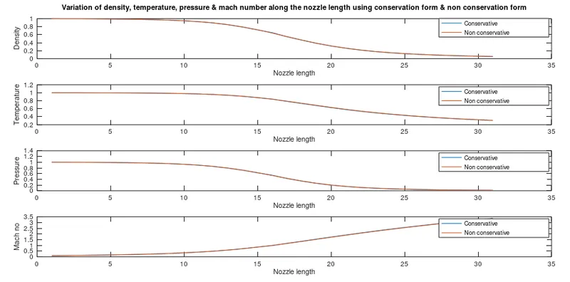
The above plot clearly shows variation is negligible in the computed primitive variables along the nozzle by using conservative and non conservative governing equations
Timewise variation of the primitive variables at the throat section:
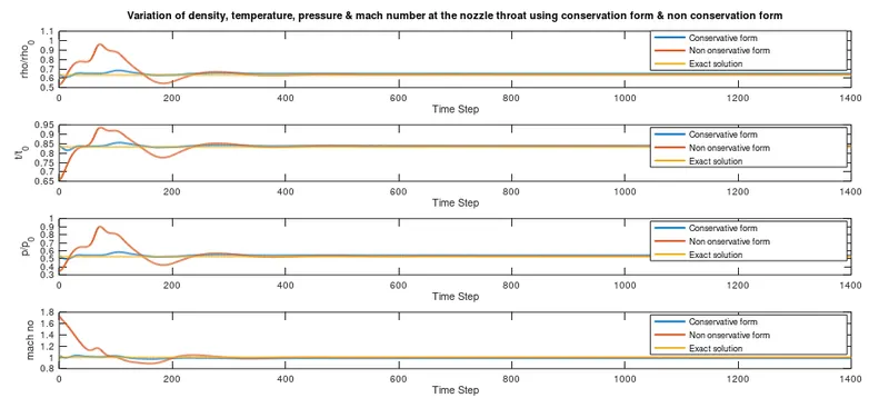
| `rho/(rhooverset(0)` | `T/(Toverset(0)` | `p/(poverset(0)` | `M` | |
| Exact Values | 0.634 | 0.833 | 0.528 | 1 |
| Non Conservation-31 grid points | 0.639 | 0.836 | 0.534 | 0.999 |
| Conservation-31 grid points | 0.649 | 0.839 | 0.545 | 0.984 |
From the above plot and the table, we can conclude non-conservative form gives more accurate results when compared to the conservative form due to error accumulation because of its complex calculation.
Mass flow rate at random timesteps by conservative form and non-conservative form:
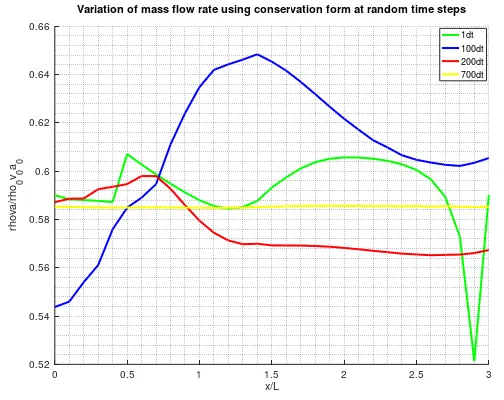
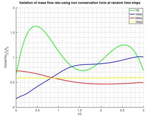
Mass flow rate from both forms governing equations in comparison with exact
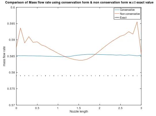
The above plots for mass flow rate show conservation form give a better result compared to non-conservative form because the mass flow rate is the primary result in conservation form but in the nonconservative form, it is computed as a secondary result.
Mass flow rate from both forms governing equations in comparison with exact
The above plots for mass flow rate show conservation form give a better result compared to non-conservative form because the mass flow rate is the primary result in conservation form i.e U2 but in the nonconservative form, it is computed as a secondary result.
Grid Independence Test:
| `rho/(rhooverset(0)` | `T/(Toverset(0)` | `p/(poverset(0)` | `M` | |
| Exact Values | 0.634 | 0.833 | 0.528 | 1 |
| Non Conservation-31 grid points | 0.639 | 0.836 | 0.534 | 0.999 |
| Non Conservation-61 grid points | 0.637 | 0.835 | 0.533 | 0.999 |
| Conservation-31 grid points | 0.649 | 0.839 | 0.545 | 0.984 |
| Conservation-61 grid points | 0.638 | 0.835 | 0.533 | 0.999 |
The above table shows by increasing the grid points to 61 give a close result using the conservative form. But non conservative form performs better by gives the same result without doubling the grid point.
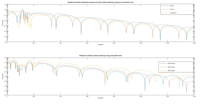
The above plot shows the residuals for the conservation form is not as good as that for the nonconservation form of the equation. In nonconservation form residuals decay upto 10e-6 after 1400 timesteps but conservation form decay 10e-3 at 1400 timesteps.
Conclusion:
1. Conservation form yields a better mass flow distribution
2. Nonconservation form leads to smaller residuals.
3. Conservative form requires more computational effort compared with non conservative form.