Simulation of a 1D Super-sonic nozzle flow simulation using Macormack Method

Objective:

To simulate the isentropic flow through a quasi 1D subsonic-supersonic nozzle using Non-conservation and Conservation forms of the governing equations and solve them using Macormack's Method/

Description:

We consider steady, isentropic flow through a convergent-divergent nozzle. The flow at the inlet to the nozzle comes from a reservoir where the pressure and temperature are denoted by `rho_0` and `T_0` respectively.

The cross-sectional area of the reservoir is large and hence the velocity is very small.

The flow is locally subsonic in the convergent section of the nozzle, sonic at the throat, and supersonic at the divergent section.

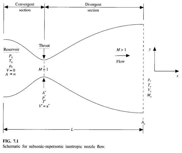
Let us consider small control of the nozzle as shown

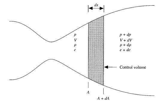
We assume that at a given section, where the cross-sectional area is A, the flow properties are uniform across the section. Hence, although the area of the nozzle changes as a function of distance along with the nozzle, x, and therefore in reality the flow filed is two-dimensional, we make the assumption that the flow properties vary only with x; this is tantamount to assuming uniform flow properties across any given cross-section. Such flow is defined as quasi-one-dimensional flow.

The governing continuity, momentum, and energy equations in terms of non-dimensional variables for this quasi-one-dimensional, steady, isentropic flow can be expressed, respectively as

Non-Conservative Continuity equation:

`(delrho')/(delt') = -rho'((delV')/(delx')) - rho'V'((del(ln A'))/(delx')) - V'((delrho')/(delx'))`

Non-Conservative Momentum equation:

`(delV')/(delt') = -V'((delV')/(delx')) -(1/gamma)((delT')/(delx') + (T')/(rho')((delrho')/(delx')))`

Non-Conservative Energy equation:

`(delT')/(delt') = -V'((delT')/(delx')) - (gamma -1)T'[(delV')/(delx') + V'(del(lnA'))/(delx')]`

Conservative Continuity equation:

`(del(rho'A'))/(delt') + (del(rho'A'V'))/(delx') = 0`

Conservative Momentum equation:

`(del(rho'A'V'))/(delt') + (del[rho'A'(V')^2 +(1/gamma)rho'A'])/(delx') = (1/gamma)rho'((delA')/(delx'))`

Conservative Energy equation:

`(del[rho'((e')/(gamma-1) + (gamma/2)(V')^2)A'])/(delt') + (del[rho'((e')/(gamma-1) + (gamma/2)(V')^2)V'A' + rho'A'V'])/(delx') = 0`

Gamma at standard air condition `gamma=1.4`

Macormack's Method

Let f(x) is the equation to be solved. Then the following steps are followed.

1. Initial profile

Before the calculation, the initial profile for all flow field variables which are density, velocity, and temperature has to be determined.

These are guess values but should be specified with more awareness of the problem.

2. Predictor step

`((delf)/(dt))_p = (f(i+1) - f(i))/(Deltax`

3. Solution update

`f_p = f_(Initial) + ((delf)/(delt))_p * Deltat`

`f_p` - Flow filed variable calculated after the predictor step

`f_(Initial)` - Flow field variable in the initial st`

`Deltat` - Time ste`

4. Corrector step

`((delf_p)/(dt))_c = (f(i) - f(i-1))/(Deltax`

`((delf)/(dt))_(avg) = 0.5(((delf)/(dt))_p +((delf_p)/(dt))_c )`

5. Final solution update

`f_(sol) = f_(Initial) + ((delf)/(delt))_(avg) * Deltat`

`f_(sol)` - Final solution of the flow field variable for the first time step

MATLAB coding:

Main coding

% Quassi 1D Supersonic Nozzle Flow using Macormack's Method
clear all
close all
clc

% Defining geometry & meshing
% Number of grid points
disp('Enter the number of nodes')
nx = input('Nodes = ');

%  Length of domain
disp('Enter the length of domain where a and b are strating and end points respectively')
a = input('Enter starting point a = ');
b = input('Enter end point b = ');

% Meshing
x=linspace(a,b,nx);

% Grid spacing
dx=x(2)-x(1);

% Area of nozzle
A=1+2.2*(x-1.5).^2;

disp('Enter the value for gamma')
gamma = input('gamma = ');

% Time step
%disp('Enter the number of time steps')
nt = 1400; %input('nt = ');

% Courant number time step control
C=0.5; 

% calling function for non conservative form
tic
[rho1,T1,V1,P1,M1,m1,rho_throat1,V_throat1,T_throat1,P_throat1,M_throat1,residual1]=Quasi_1D_nozzle_flow_non_conservative_func(x,dx,A,C,nt,gamma);
Time_taken_by_non_conservative_form=toc

% calling function for conservative form
tic
[rho2,T2,V2,P2,M2,m2,rho_throat2,V_throat2,T_throat2,P_throat2,M_throat2,residual2]=Quasi_1D_nozzle_flow_conservative_func(x,dx,A,C,nt,gamma);
Time_taken_by_conservative_form=toc

%plots for different variables
%plots for different flow parameters:non conservative form

 figure(1)
 subplot(4,1,1)
 plot(x,M1,'linewidth',2)
 grid on
 grid minor;
 ax=gca;
 ax.FontSize=8;
 ylim([0,4.5])
 yticks(0:1.5:4.5)
 ylabel('Mach number','Fontsize',8,'FontWeight','bold')
 title('Non-conservative form of lowering equation','Fontsize',12,'FontWeight','bold','color','black')
 
 subplot(4,1,2)
 plot(x,P1,'linewidth',2)
 grid on
 grid minor;
 ax=gca;
 ax.FontSize=8;
 yticks(0:0.2:1);
 ylabel('Pressure ratio','Fontsize',8,'FontWeight','bold')
 
 subplot(4,1,3)
 plot(x,rho1,'linewidth',2)
 grid on
 grid minor;
 ax=gca;
 ax.FontSize=8;
 yticks(0:0.2:1);
 ylabel('Density ratio','Fontsize',8,'FontWeight','bold')
 
 subplot(4,1,4)
 plot(x,T1,'linewidth',2)
 grid on
 grid minor;
 ax=gca;
 ax.FontSize=8;
 ylim([0,1]);
 yticks(0:0.2:1);
 ylabel('Temperature ratio','Fontsize',8,'FontWeight','bold')
 xlabel('x/L','Fontsize',12,'FontWeight','bold')

%plots for different flow parameters: conservative form
figure(2)
subplot(4,1,1)
plot(x,M2,'linewidth',2)
grid on
grid minor;
ax=gca;
ax.FontSize=8;
ylim([0,4.5])
yticks(0:1.5:4.5)
ylabel('Mach number','Fontsize',8,'FontWeight','bold')
title('Conservative form of lowering equation','FontSize',12,'FontWeight','bold','color','black')

subplot(4,1,2)
plot(x,P2,'linewidth',2)
grid on
grid minor;
ax=gca;
ax.FontSize=8;
yticks(0:0.2:1);
ylabel('Pressure ratio','Fontsize',8,'FontWeight','bold')

subplot(4,1,3)
plot(x,rho2,'linewidth',2)
grid on
grid minor;
ax=gca;
ax.FontSize=8;
yticks(0:0.2:1);
ylabel('Density ratio','Fontsize',8,'FontWeight','bold')

subplot(4,1,4)
plot(x,T2,'linewidth',2)
grid on
grid minor;
ax=gca;
ax.FontSize=8;
ylim([0,1]);
yticks(0:0.2:1);
ylabel('Temperature ratio','Fontsize',8,'FontWeight','bold')
xlabel('x/L','Fontsize',8,'FontWeight','bold')

%plots for different flow parameters at throat section:non-conservative vs
%conservative form
figure(3)
subplot(4,1,1)
plot(1:nt,M_throat1,'Linewidth',2)
hold on
plot(1:nt,M_throat2,'Linewidth',2)
grid on
grid minor
ax=gca;
ax.FontSize=8;
yticks(0:0.2:1)
ylabel('Mach Number','FontSize',8,'FontWeight','bold')
l_g_d=legend('Non-conservative','Conservative');
l_g_d.FontSize=8;
title('Throat section of nozzle','FontSize',12,'FontWeight','bold','color','black')

subplot(4,1,2)
plot(1:nt,P_throat1,'Linewidth',2)
hold on
plot(1:nt,P_throat2,'Linewidth',2)
grid on
grid minor
ax=gca;
ax.FontSize=8;
yticks(0:0.2:1)
ylabel('P/P_0','FontSize',8,'FontWeight','bold')
l_g_d=legend('Non-conservative','Conservative');
l_g_d.FontSize=8;

subplot(4,1,3)
plot(1:nt,rho_throat1,'Linewidth',2)
hold on
plot(1:nt,rho_throat2,'Linewidth',2)
grid on
grid minor
ax=gca;
ax.FontSize=8;
yticks(0:0.2:1)
ylabel('rho/rho_0','FontSize',8,'FontWeight','bold')
l_g_d=legend('Non-conservative','Conservative');
l_g_d.FontSize=8;

subplot(4,1,4)
plot(1:nt,T_throat1,'Linewidth',2)
hold on
plot(1:nt,T_throat2,'Linewidth',2)
grid on
grid minor
ax=gca;
ax.FontSize=8;
yticks(0:0.2:1)
ylabel('T/T_0','FontSize',8,'FontWeight','bold')
l_g_d=legend('Non-conservative','Conservative');
l_g_d.FontSize=8;

%plots for residuals:non-conservative vs conservative
figure(4)
subplot(2,1,1)
plot(1:nt,residual1,'Linewidth',2)
grid on
grid minor
ax=gca;
ax.FontSize=8;
xlabel('Time steps','FontSize',8,'FontWeight','bold')
ylabel('Residuals','FontSize',8,'FontWeight','bold')
yticks(0:0.2:1.2)
l_g_d=legend('|drho/dt|_{av}','|dV/dt|_{av}','|dT/dt|_{av}');
l_g_d.FontSize=8;
title('Residuals of non conservative form','FontSize',12,'FontWeight','bold','color','black')

subplot(2,1,2)
plot(1:nt,residual2,'Linewidth',2)
grid on
grid minor
ax=gca;
ax.FontSize=8;
xlabel('Time steps','FontSize',8,'FontWeight','bold')
ylabel('Residuals','FontSize',8,'FontWeight','bold')
yticks(0:0.5:4)
l_g_d=legend('|dU_1/dt|_{av}','|dU_2/dt|_{av}','|dU3_3/dt|_{av}');
l_g_d.FontSize=8;
title('Residuals of conservative form','FontSize',12,'FontWeight','bold','color','black')

%plots for mass flow rate variation:non-conservative form
figure(5)
plot(x,m1(50,:),'-*','Linewidth',2)
hold on
grid on
grid minor
plot (x,m1(100,:),'-x','Linewidth',2)
hold on
plot (x,m1(150,:),'-d','Linewidth',2)
hold on
plot (x,m1(200,:),'-p','Linewidth',2)
hold on
plot (x,m1(500,:),'-o','Linewidth',2)
hold on
plot (x,m1(700,:),'-s','Linewidth',2)
hold on
plot (x,m1(1400,:),'--','Linewidth',2)
xlabel('x/L','Fontsize',15,'FontWeight','bold')
ylabel('rhoAV/rho_0A*a_0','FontSize',15,'FontWeight','bold')
l_g_d=legend('50 Delta','100 Delta','150 Delta','200 Delta','500 Delta','700 Delta','1400 Delta')
l_g_d.FontSize=8;
title('variation of non-dimensional mass flow rate:non conservative form','FontSize',10,'FontWeight','bold','color','black')

%plots for mass flow rate variation:conservative form
figure(6)
plot(x,m2(50,:),'-*','Linewidth',2)
hold on
grid on
grid minor
plot (x,m2(100,:),'-x','Linewidth',2)
hold on
plot (x,m2(150,:),'-d','Linewidth',2)
hold on
plot (x,m2(200,:),'-p','Linewidth',2)
hold on
plot (x,m2(500,:),'-o','Linewidth',2)
hold on
plot (x,m2(700,:),'-s','Linewidth',2)
xlabel('x/L','Fontsize',8,'FontWeight','bold')
ylabel('rhoAV/rho_0A*a_0','FontSize',8,'FontWeight','bold')
l_g_d=legend('50 Delta','100 Delta','150 Delta','200 Delta','500 Delta','700 Delta')
l_g_d.FontSize=8;
title('variation of non-dimensional mass flow rate:conservative form','FontSize',10,'FontWeight','bold','color','black')

%plot for variation of non-dimensional mass flow rate-steady state:non
%conservative vs conservative.
figure(7)
plot(x,0.579*ones(length(x),1),'--','Linewidth',2)
hold on
grid on
grid minor
plot(x,m1(end,:),'Linewidth',2)
hold on
plot(x,m2(end,:),'Linewidth',2)
ax=gca;
ax.FontSize=8;
xlabel('x/L','Fontsize',8,'FontWeight','bold')
ylabel('rhoAV/rho_0A*a_0','FontSize',8,'FontWeight','bold')
legend('Exact','nonconservative','conservative','FontSize',8)
title('variation of non-dimensional mass flow rate:steady state','FontSize',10,'FontWeight','bold','color','black')

Function for Non-conservative form

% 1D Supersonic Nozzle Non-Conservative Eqns of 
% Continuity, Momentum, and Energy by Macormack Method
%user defined function for quasi 1-D supersonic nozzle flow
%non-conservative form of governing equation

function[rho1,T1,V1,P1,M1,m1,rho_throat1,V_throat1,T_throat1,P_throat1,M_throat1,residual1]=Quasi_1D_nozzle_flow_non_conservative_func(x,dx,A,C,nt,gamma)

%initial conditions (at time,t=0);

%density

rho_at_t_0=1-0.314*x;

%temperatue
T_at_t_0=1-0.2314*x;

%velocity
V_at_t_0=(0.1+1.09*x).*T_at_t_0.^(0.5);

rho1=rho_at_t_0;
T1=T_at_t_0;
V1=V_at_t_0;

%Mass flowrate
m1=zeros(nt,length(x));

%defining area at throat
throat=find(A==1);

%initial condition of variables at the throat section;
rho_throat1=zeros(nt,1); %denisty at throat
T_throat1=rho_throat1; %temp at throat
V_throat1=T_throat1; % velocity at throat
P_throat1=V_throat1; %pressure at throat
M_throat1=P_throat1; %mach number at throat


residual1=zeros(nt,3);

%using macCormack method
%time loop
for k=1:nt
    
    %creating a copy of old values
    rho_old=rho1;
    T_old=T1;
    V_old=V1;
    
    %stability criterion (CFL condition)
    %time-step (dt)
    dt=min(C*dx./(T1.^0.5+V1));
    
    %Predictor-step
    %space loop
    for i=2:length(x)-1
        
        %discretizing using forward difference scheme for spatial
        %derivatives
        dVdx=(V1(i+1)-V1(i))/dx;
        dlogAdx=(log(A(i+1))-log(A(i)))/dx;
        drhodx=(rho1(i+1)-rho1(i))/dx;
        dTdx=(T1(i+1)-T1(i))/dx;
        
        %continuity equation 
        drho_dt_p(i)=-rho1(i)*dVdx-rho1(i)*V1(i)*dlogAdx-V1(i)*drhodx;
        
        %momentum equation
        dV_dt_p(i)=-V1(i)*dVdx-(1/gamma)*(dTdx+(T1(i)/rho1(i))*drhodx);
        
        %energy equation
        dT_dt_p(i)=-V1(i)*dTdx-(gamma-1)*T1(i)*(dVdx+V1(i)*dlogAdx);
        
        %interim solution update
        rho1(i)=rho1(i)+drho_dt_p(i)*dt;
        V1(i)=V1(i)+dV_dt_p(i)*dt;
        T1(i)=T1(i)+dT_dt_p(i)*dt;
        
    end %end of space loop (predictor-step)
    
    %corrector-step
    %space loop
    for i=2:length(x)-1
        
          %discretizing using backward difference scheme for spatial
          %derivatives
          dVdx=(V1(i)-V1(i-1))/dx;
        dlogAdx=(log(A(i))-log(A(i-1)))/dx;
        drhodx=(rho1(i)-rho1(i-1))/dx;
        dTdx=(T1(i)-T1(i-1))/dx;
        
          %continuity equation 
        drho_dt_c(i)=-rho1(i)*dVdx-rho1(i)*V1(i)*dlogAdx-V1(i)*drhodx;
        
        %momentum equation
        dV_dt_c(i)=-V1(i)*dVdx-(1/gamma)*(dTdx+(T1(i)/rho1(i))*drhodx);
        
        %energy equation
        dT_dt_c(i)=-V1(i)*dTdx-(gamma-1)*T1(i)*(dVdx+V1(i)*dlogAdx);
        
    end % end of spaace loop (corrector-step)
    
    
    
    %computing average time derivative
    drho_dt=0.5*(drho_dt_p+drho_dt_c);
    dV_dt=0.5*(dV_dt_p+dV_dt_c);
    dT_dt=0.5*(dT_dt_p+dT_dt_c);
    
    residual1(k,1)=max(abs(drho_dt));
      residual1(k,2)=max(abs(dV_dt));
        residual1(k,3)=max(abs(dT_dt));
        
        %final solution update
        for j=2:length(x)-1
            rho1(j)=rho_old(j)+(drho_dt(j)*dt);
            V1(j)=V_old(j)+(dV_dt(j)*dt);
            T1(j)=T_old(j)+(dT_dt(j)*dt);
        end
        
        %Applying boundary conditions
        %subsonic inflow boundary;
        V1(1)=2*V1(2)-V1(3); %velcoity at inlet
        
        %supersonic outflow boundary
        V1(end)=2*V1(end-1)-V1(end-2); %velocity at outlet
        rho1(end)=2*rho1(end-1)-rho1(end-2); %density at outlet
        T1(end)=2*T1(end-1)-T1(end-2); %temperature at outlet
        
        %mass flow rate
        m1(k,:)=rho1.*A.*V1;
        
        %pressure
        P1=rho1.*T1;
        
        %mach number
        M1=V1./(T1.^0.5);
        
        %values at throat
        rho_throat1(k)=rho1(throat);
        M_throat1(k)=M1(throat);
        P_throat1(k)=P1(throat);
        T_throat1(k)=T1(throat);
        V_throat1(k)=V1(throat);
end %end of time loop
end %end of function

Function for conservative form

% 1D Supersonic Nozzle Conservative Eqns of 
% Continuity, Momentum, and Energy by Macormack Method
%user defined function for quasi 1-D supersonic nozzle flow
%conservative form of governing equation

function[rho2,T2,V2,P2,M2,m2,rho_throat2,V_throat2,T_throat2,P_throat2,M_throat2,residual2]=Quasi_1D_nozzle_flow_conservative_func(x,dx,A,C,nt,gamma)

%initial conditions (at time,t=0);
rho_at_t_0=zeros(1,length(x));
T_at_t_0=rho_at_t_0;
V_at_t_0=T_at_t_0;

for i=1:length(x)
    if x(i)>=0 && x(i)<0.5
        rho_at_t_0(i)=1;
        T_at_t_0(i)=1;
        
        
    elseif x(i)>=0.5 && x(i)<1.5
        rho_at_t_0(i)=1-0.366*(x(i)-0.5);
        T_at_t_0(i)=1-0.167*(x(i)-0.5);
        
    elseif x(i)>=1.5 && x(i)<=3.5
          rho_at_t_0(i)=0.634-0.3879*(x(i)-1.5);
        T_at_t_0(i)=0.833-0.3507*(x(i)-1.5);
        
    end
    
    V_at_t_0(i)=0.59/(rho_at_t_0(i)*A(i));
end

rho2=rho_at_t_0;
T2=T_at_t_0;
V2=V_at_t_0;

%mass flow rate 
m2=zeros(nt,length(x));

%initial conditions for the solution vectors
U1=rho2.*A;
U2=rho2.*A.*V2;
U3=rho2.*A.*((T2./(gamma-1))+(gamma/2).*(V2.^2));

%defining area at throat
throat=find(A==1);

%initial conditions variables at the throat section
rho_throat2=zeros(nt,1);
T_throat2=rho_throat2; %temp at throat
V_throat2=T_throat2; % velocity at throat
P_throat2=V_throat2; %pressure at throat
M_throat2=P_throat2; %mach number at throat


residual2=zeros(nt,3);

%using macCormack method
% time loop
for k=1:nt
    
    %creating a copy of old values
    U1_old=U1;
    U2_old=U2;
    U3_old=U3;
    
    %stability criterion (CFL condition)
    %time-step(dt)
    dt=min(C*dx./(T2.^0.5+V2));
    
    
    %initial conditions for flux vectors (F)
    F1=U2;
    F2=(U2.^2)./U1+((gamma-1)/gamma)*(U3-0.5*gamma*(U2.^2)./U1);
    F3=gamma*U2.*U3./U1-0.5*gamma*(gamma-1)*(U2.^3)./(U1.^2);
    
    %predictor step
    %space loop
    for i=2:length(x)-1
        %discretizing usingforward difference scheme for spatial
        %derivatives
        %source vector
        J2=(1/gamma)*rho2(i)*T2(i)*((A(i+1)-A(i))/dx);
        
        %continuity equation
        dU1_dt_p(i)=-(F1(i+1)-F1(i))/dx;
        
        %momentum equation
        dU2_dt_p(i)=-(F2(i+1)-F2(i))/dx+J2;
        
        % energy equation
        dU3_dt_p(i)=-(F3(i+1)-F3(i))/dx;
        
        %interim solution update
        
        U1(i)=U1(i)+dU1_dt_p(i)*dt;
         U2(i)=U2(i)+dU2_dt_p(i)*dt;
          U3(i)=U3(i)+dU3_dt_p(i)*dt;
          
    end
    
    %obtaining the primitive variables form our solution vector (U1,U2,U3);
    rho2=U1./A;
    V2=U2./U1;
    T2=(gamma-1)*((U3./U1)-((gamma/2)*(V2.^2)));
    
    %updating flux vectors
    F1=U2;
    F2=((U2.^2)./U1)+(((gamma-1)/gamma)*(U3-((gamma/2)*(U2.^2./U1))));
    F3=((gamma.*U2.*U3)./U1)-((gamma*(gamma-1))/2)*(U2.^3)./(U1.^2);
    
    %corrector step
    %space loop
    for i=2:length(x)-1
        %discretizing using backward difference scheme for spatial
        %derivatives
        %sourve vector
        J2=(1/gamma)*rho2(i)*T2(i)*((A(i)-A(i-1))/dx);
        
        %continuity equation
        dU1_dt_c(i)=-(F1(i)-F1(i-1))/dx;
        
        %momentum equation
         dU2_dt_c(i)=-(F2(i)-F2(i-1))/dx+J2;
         
         %energy equation
         dU3_dt_c(i)=-(F3(i)-F3(i-1))/dx;
         
    end
    
    %computing the average time derivative
    dU1_dt=0.5*(dU1_dt_p+dU1_dt_c);
    dU2_dt=0.5*(dU2_dt_p+dU2_dt_c);
    dU3_dt=0.5*(dU3_dt_p+dU3_dt_c);
    
    residual2(k,1)=max(abs(dU1_dt));
    residual2(k,2)=max(abs(dU2_dt));
    residual2(k,3)=max(abs(dU3_dt));
    
    % final solution update
    for j=2:length(x)-1
        U1(j)=U1_old(j)+dU1_dt(j)*dt;
        U2(j)=U2_old(j)+dU2_dt(j)*dt;
        U3(j)=U3_old(j)+dU3_dt(j)*dt;
    end
    
    %subsonic inflow boundary
    U1(1)=rho2(1)*A(1);
    U2(1)=2*U2(2)-U2(3);
    
    U3(1)=U1(1)*((T2(1)/(gamma-1))+0.5*gamma*V2(1)^2);
    
    %supersonic outflow boundary
    U1(end)=2*U1(end-1)-U1(end-2);
    U2(end)=2*U2(end-1)-U2(end-2);
    U3(end)=2*U3(end-1)-U3(end-2);
    
    
    %final values of different variables;
    rho2=U1./A;
    V2=U2./U1;
    T2=(gamma-1)*((U3./U1)-0.5*gamma*V2.^2);
    M2=V2./(T2.^0.5);
    P2=rho2.*T2;
    m2(k,:)=rho2.*A.*V2; %mass flow rate
    
    rho_throat2(k)=rho2(throat);
    V_throat2(k)=V2(throat);
    T_throat2(k)=T2(throat);
    P_throat2(k)=P2(throat);
    M_throat2(k)=M2(throat);
    
end %end of the time loop
end %end of the function

Command window:

Node = 31

Node = 61

Output and results:

Non-cons	cons	Non-cons	cons	Non-cons	cons	Non-cons	cons	Non-cons	cons
0	0	0.098782	0.98348	1	1	1	1	1	1
0.5	0.5	0.18703	0.18564	0.98232	0.98288	0.98734	0.98769	0.99429	0.99513
1	1	0.41552	0.41592	0.89547	0.89377	0.92414	0.92288	0.96896	0.96846
1.5	1.5	0.99937	0.98173	0.53424	0.54635	0.63869	0.65039	0.83646	0.84005
2	2	1.8901	1.9081	0.15316	0.15316	0.26184	0.25967	0.58495	0.57992
2.5	2.5	2.6963	2.7149	0.043785	0.043785	0.10721	0.10582	0.4084	0.40503
3	3	3.3532	3.367	0.016295	0.016295	0.052857	0.052717	0.30827	0.30549

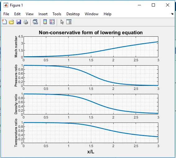
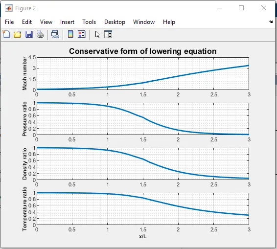
From the above plot and the data, we can notice that as the Mach number increases flow reaches from subsonic to the supersonic regime. The primitive variables such as density, pressure, and temperature show de-activity after the sonic region (Mach=1), till the exit of the nozzle. Although, these results are almost identical to the analytical solution. Results validated from the CFD book by John D Anderson.

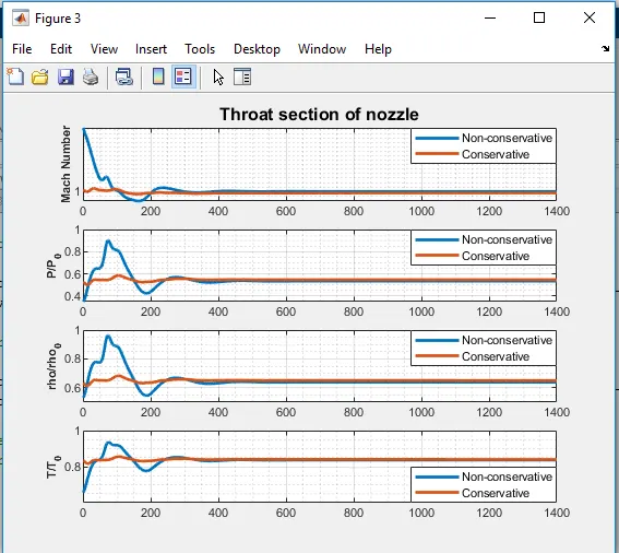
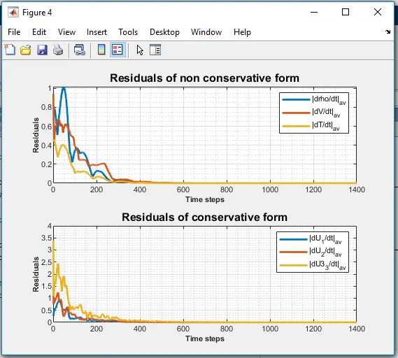
From the above plot- variation of different primitive variables w.r.t time step, we can see that the conservative form which can be used to modify initial conditions converges to steady-state faster than the non-conservative form.

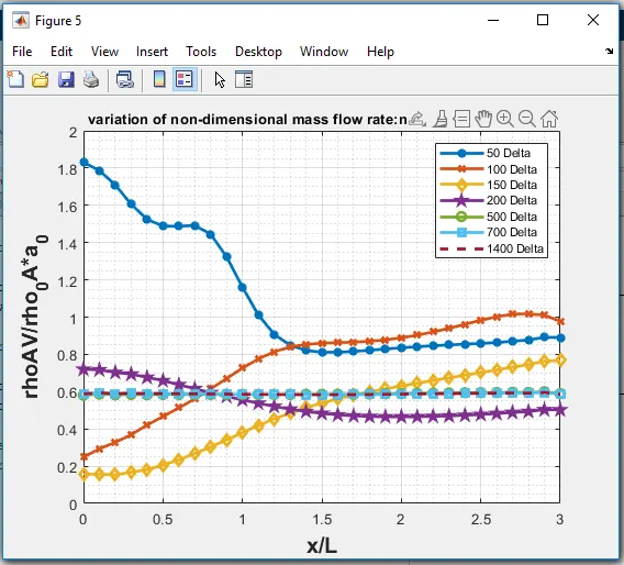
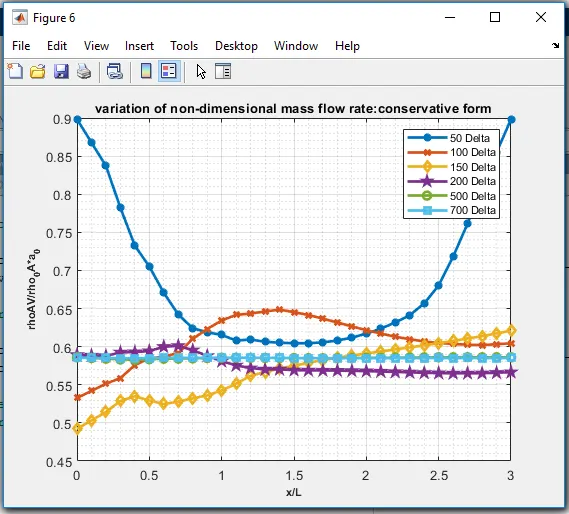
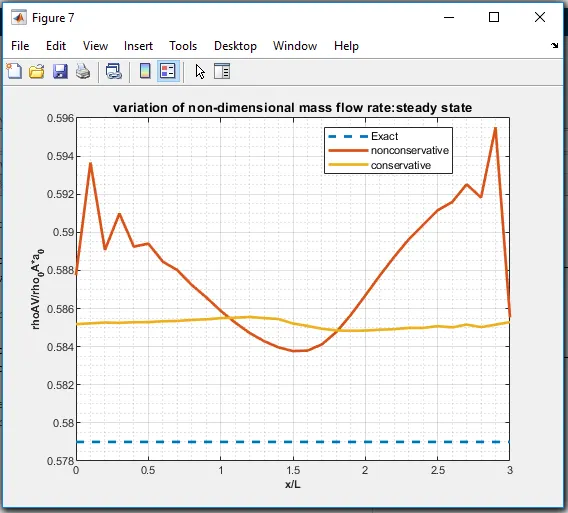
In the above plot, we compare the steady-state variation of mass flow obtained with the non-conservative and conservative forms of the governing equations. Here we see that the steady-state mass flow distribution predicted by the conservative form of the equation is much more satisfactory than from the obtained non-conservative form on two accounts.

1. The conservative form gives the distribution which is much closer to being a constant. In contrast, the non-conservative results have sizable variations with some oscillations at both inflow and outflow boundary of course on a partial basis, these variations are not apart and the mass flow essentially appears to be constant.

2.The steady-state mass flow results obtained with the conservative forms are, on the whole much closer to exact analytical solutions (Rho ’A V’= 0.579).

Grid dependency test:

Grid dependency test	rho/rho0	T/To	P/Po	M
exact analytical solution	0.634	0.833	0.528	1.00
non-conservative form 31 grid points	0.6387	0.8365	0.5342	0.9994
conservative form 31 grid points	0.6504	0.8401	0.5465	0.9817
non-conservative form 61 grid points	0.6376	0.8354	0.5326	0.9997
conservative form 61 grid points	0.6382	0.8352	0.5330	0.9993

The above discussion does not necessarily establish a definite superiority of the conservative form results over the non-conservative form result, let us look at the primitive variables in particular density, temperature, pressure, and Mach number at nozzle throat as tabulated in the above table. By doubling the number of grid points the steady-state numerical results are slightly closer to the exact, analytical values. for all the particular purposes we have grid independence with 31 grid points sufficient to produce the steady-state results.

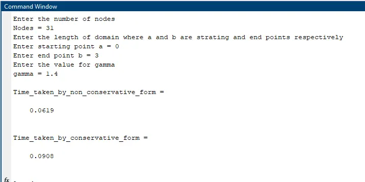
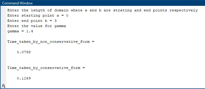
The time taken for non-conservative form 31 grid points is 0.0619sec and for 61 grid points =0.0798 sec.

The time taken for conservative form 31 grid points is 0.0908sec and for 61 grid points =0.1269sec.

There are three reasons for the small numerical inaccuracy (residue).

They are: -

Small Inflow Boundary Condition Error: Initially we assumed that the density, temperature, and pressure at the inlet were equal to reservoir properties. This will be only true if the Mach number at the inlet is equal to zero. But Mach number is a function of the area ratio A/A*. Even at the inlet, finite values exist for the area ratio (5.95), and hence there must be a finite Mach number at the inlet (x=0), both numerically and analytically. It is a built-in error and is not viewed as serious.

Courant Number Effect: According to the Courant Number Stability Criteria, the CFL number must be less than or equal to 1. But here we assumed C=0.5 which is smaller than the necessary, at which the solution is stable and the results are closer to the exact analytical solution. So, we can conclude that we made a safe guess. CFL criteria provide a good estimate to calculate the time step value for even the non-linear hyperbolic partial differential equation (Quasi 1D nozzle flow), but it does not exactly hold good as it is derived for the linear hyperbolic equation.

Grid Dependence: Even if the number of grid points is doubled, and there is only a marginal difference in the solution, then our original calculation with the initial number of grid points is said to be grid-independent. This factor is purely based on the circumstances, by depending upon the expected order of accuracy and the allowable range of tolerance.