Week 7: Shock tube simulation project

Shock tube simulation

Objectives:

To set up a transient shock tube simulation using Converge CFD and plot;

1. Pressure and temperature history in the entire domain

2. Cell count as a function of time

Shock Tube:

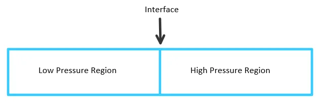
• A shock tube is a device that is used to produce confined shock waves. It contains a diaphragm (interface) that separates a high pressure and a low-pressure region. When the pressure ratio between the two sections is maintained at desired levels and the diaphragm is ruptured, a shock wave propagates.
• It creates a compression wave that propagates to the low-pressure section and expansion waves which traverse in the high-pressure section. After a short interval of time, the compression waves in the low-pressure region will merge to form a shock wave. The stationary gases in the low-pressure area will experience a rise in pressure and temperature due to the formation of shock waves and they will start moving towards the walls of the tube. Since the shock wave travels at supersonic speeds, it generates an expansion wave called an expansion fan.
• An expansion fan consists of an infinite number of mach waves that diverge from a sharp corner. Both the expansion fan and the shock waves are reflected from the closed ends of the tube. When the shock wave hits the closed end of the tube, it gets reflected back. This reflected shock wave cancels the motion of the gases in the low-pressure section initiated by the primary shock wave. The strength of the shock wave and expansion fan depends on the initial pressure ratio across the diaphragm and the physical properties of the gases present in the tube.
• By replicating the flow of gases in the presence of a shock wave, parameters such as rates of chemical kinetics, dissociation energies, etc.

Geometry:

The geometry of the shock tube measures a length of 0.2m which is divided into the Low-Pressure region consisting of O2 and the High-Pressure region consisting of N2.

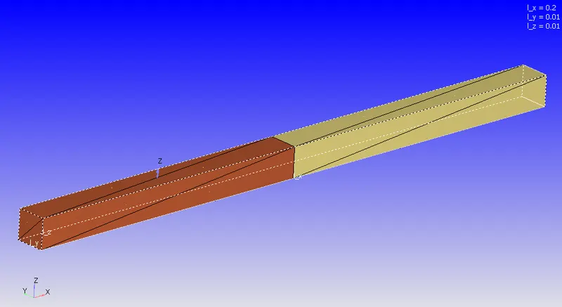
Simulation type: Transient

Turbulence model: OFF

Solver: PISO (Density-based)

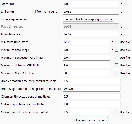
Simulation time parameters:

The total time period in the simulation is set to 0.012 seconds with the initial time step and a maximum time step of 1e-09s and 1s respectively.

Boundary & Initial conditions:

Zone	BC	IC
LP (O2)	Slip Wall	101325 Pa, Mass Fraction of O2 = 1
HP (N2)	Slip Wall	600000 Pa, Mass Fraction of N2 = 1

Events:

Events are applied to perform certain movements such as opening or closing of any desired regions. Here it is applied to initiate the rupture of the diaphragm such that both the regions come into contact to form a shock due to pressure variations. The below image shows that at t=0s, both the regions are intact whereas at t=0.001s, regions are open for contact which in the real world is the rupture of the diaphragm.

Meshing: (Click here)

The base grid is set to 0.004m which is further coupled with Adaptive Mesh Refinement.

Adaptive Mesh Refinement:

Adaptive Mesh Refinement of embed scale 3 is applied to N2 species. This ensures that the region where there is a presence of N2 is refined well enough to capture the shock profile. In the below image, the embed scale of 3 levels is highlighted as L1, L2, and L3.

Results:

Velocity Profile:(Click here)

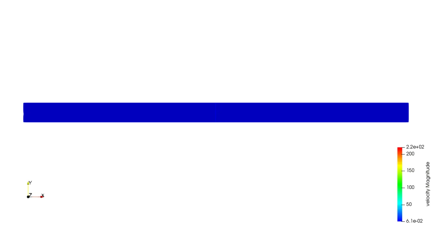
Initially high magnitude of velocity propagates from the center of the shock tube due to rupture of the diaphragm. Further, the velocity variation settles down as the shock wave gets neutralized.

Pressure Profile: (Click here)

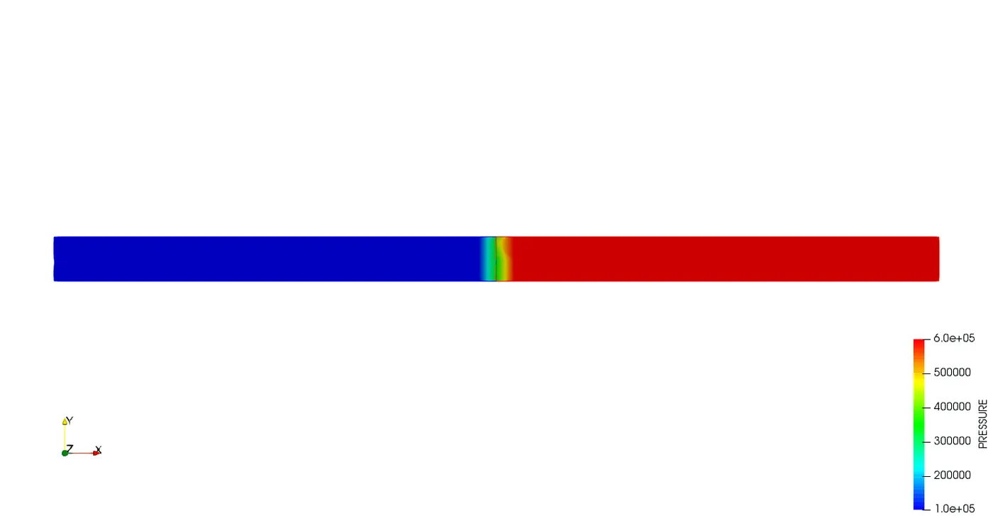
Initially, the N2 region is initialized with a higher pressure of 6bar (0.6 MPa). When the diaphragm is ruptured by the event defined in the solver at 0.001s, the pressure contained in the N2 region gets propagated into the low-pressure region (O2). This abrupt change in pressure leads to the shock wave.

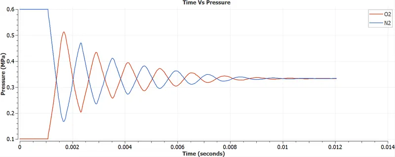
The formation of shock waves is evident from the plot below which shows the oscillations of pressure at both regions. The high-pressure species N2 experiences a steep decrease whereas the low-pressure species O2 experiences a steep increase. This phenomenon repeats but the magnitude of variation reduces subsequently settling to a value of around 0.3 Mpa. Once both the species reach a similar magnitude, the shock wave gets neutralized leading to a stable fluid volume with no variation of pressure.

Temperature Variation:

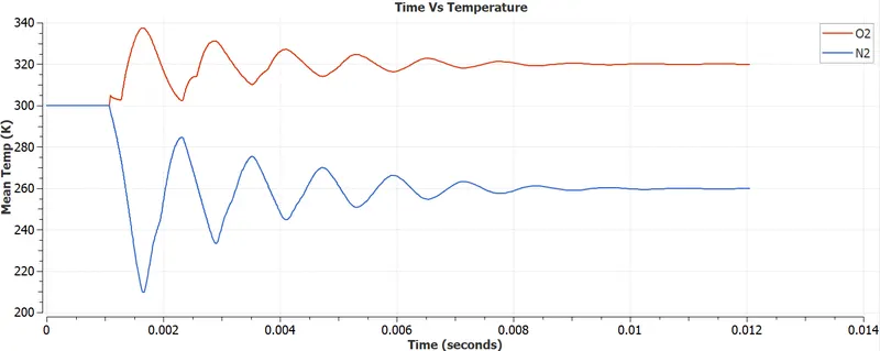
Both the regions are initialized with an initial value of 300K but at different pressures of 0.1 MPa for O2 and 0.6 MPa for N2. The above plot shows the final temperature of both species after the elimination of shock waves.

Total Cell count: (Click here)

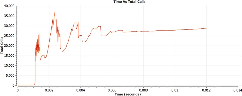
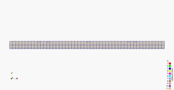
From the above plot, it is evident that the cell count is varying with respect to time. This is due to the Adaptive Mesh Refinement applied to N2 species. Whenever the N2 species is expanded or compressed (here expansion is dominant as it is in higher pressure), there is a variation of cell count with respect to time as shock propagates. But after a certain time period of around 0.006s, the shock gets normalized and the cell variation does not happen abruptly.

The below animation correlates to the above plot. The movement of finer cells indicates the N2 species. The N2 species expands and hits the walls, and then it returns back with huge expansion leading to extra cells. This leads to a variation in the number of cells with respect to time.

Inferences:

• The variation of pressure with respect to time occurs like a harmonic pattern between both the species, N2 and O2. Later, it settles down to a constant value with almost zero gradients.
• When AMR is used, cell count varies with respect to time. The variation of cells occurs around the species to which it is applied and the variation of count depends on the movement of that particular species.
• The temperature of the species also varies abruptly during the shock phase, later settles down to a magnitude based on the pressure conditions to which they are neutralized.
• The velocity of species at higher pressure increases abruptly at the initiation of shock as the pressure tends to lesser magnitude.