Shock tube simulation project
Objective:
- Setup a transient shock tube simulation
- Plot the pressure and temperature history in the entire domain
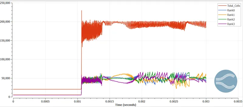
- Plot the cell count as a function of time
Solution:
Here we have a .STL file of a rectangular channel and where we simulate the flow and learn the concept of regions and events in converge CFD. Shock tube problems are mainly used to study the chemical kinetics of the reaction in a flow. Here we are going to have two regions in a simulation, 1st is the High-pressure region, and the other low-pressure region. Our objective is to engineer the flow to be in motion from high to a low zone using a particular tool called EVENTS. where we set up commands that allow shock flow-through diaphragm in between them. which separates them. The diaphragm is actually broken which will develop in shock waves. And due to high temperature between the zones Autoignition takes place that allows us to calculate ignition delay, a data which is very useful in comparing results are obtained.
Theory:
Shock tubes have been employed by a number of shock wave researchers as the most reliable facility for investigating the structure of a shock wave, shock wave propagation and reflection, and so on, because their operation principle is surprisingly very simple. Vieille (1899, 1970) described shock tube experiments in 1899, and his work today is recognized as the first published paper on shock tube flows. In his experiments, he divided a cylindrical tube into two parts by a diaphragm and obtained a discontinuity (shock wave) with a speed over 600 m/s by rupturing the diaphragm with a high-pressure gas that was supplied into one side. This type of facility is still used at present as a fundamental type of shock tube (Fig. 1). The effect of the diaphragm thickness on the discontinuity speed was investigated by varying the rupturing pressure using collodion diaphragms of 0.29 and 0.11 mm in thickness and a paper diaphragm. Further, Vieille attempted to increase the propagation speed of the discontinuity by using a driver section with a larger volume but keeping the diaphragm thickness the same. The result showed that the propagation speed was independent of the volume of the driver section, which today is explained by shock tube theory. In memory of his pioneering work, an invited paper titled “Paul Vieille Lecture” is being presented at the meetings of the international symposia on shock tubes and waves.

 fig 1
fig 1So the objective is to perform a flow simulation where we monitor the flow and analyze the YN2 species and Velocity in that regions. we need to monitor every parameter while the flow is going.
Case Setup:
Now here we start by running the COnverge CFD software were building up a case setup of channel flow that represents the parameters to run the data. No where we already have a .STL file so we download it grab the file and drag it to the converge or you can do with the conventional method by opening new projects in the new section. But here we have this block.
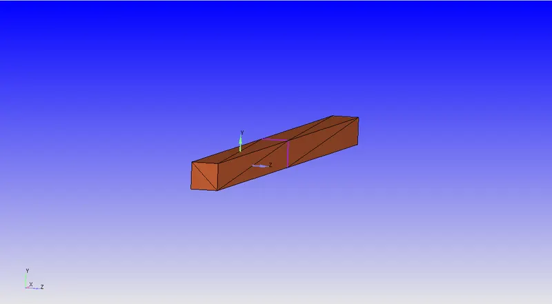
Now we have to assign boundaries to block. Here we can see that converge cfd the 2d walls is recognizable and case setup crashes while running simulation. Here while assigning the boundaries we cover one half full for high pressure and another for full low pressure region. You can also toggle the NORMALS to view the normals on the geometry to view the flow motions.
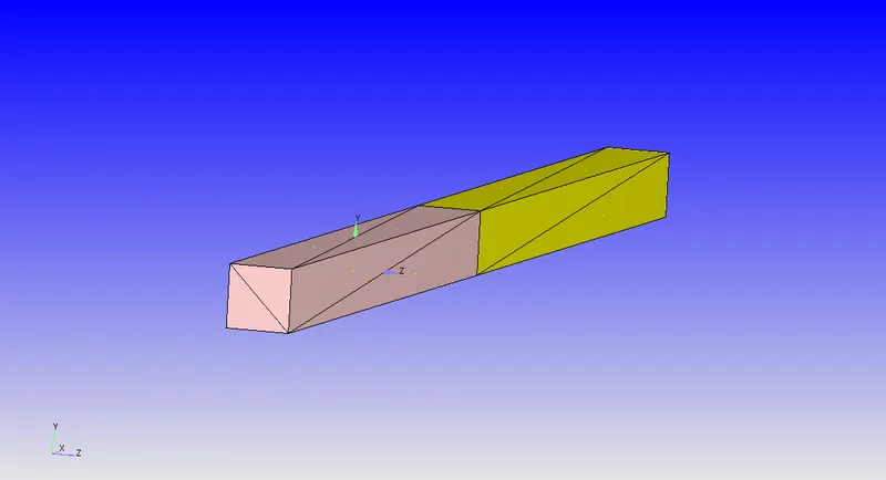
Now that we have geometry set along with boundaries to be assigned as HIGH PRESSURE and LOW PRESSURE , we can forward for the case setup now. Now the Assigning all types of Technical parameters for the flow property to case set up in the bottom right side. Below is the image is shown where all the case setup should like. The green tick indicates the all the parameter is set right according to flow properties. We can view this as below.
Assigning the boundaries is must so that converge can recognize which is which to begin and understand the case setup part.
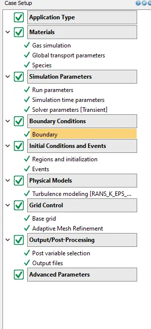
Before Jumping into the simulation part in Cygwin, one needs to set up the parameters in case set up to look like the above image. The value represents in the above image shows the completion of the properties, here's how every section needs to be done.
Application type:
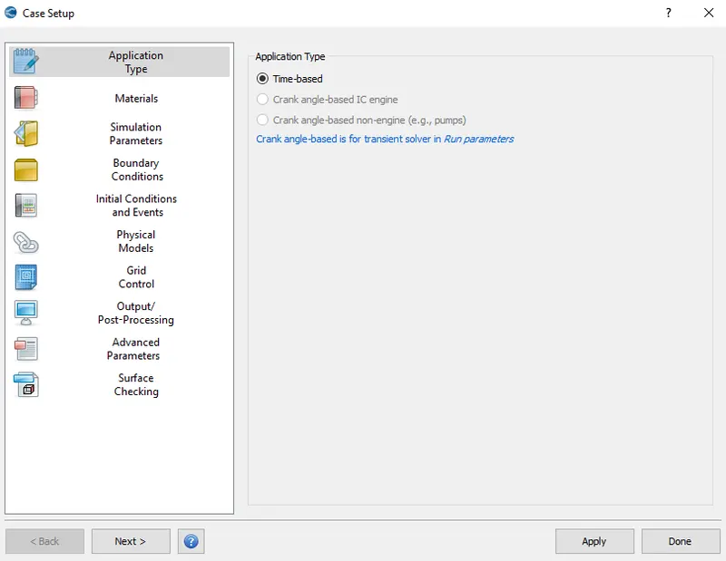
Selecting the Time-Based is the option available here as we are only setting up a simple channel flow profile, to begin with.
Materials:
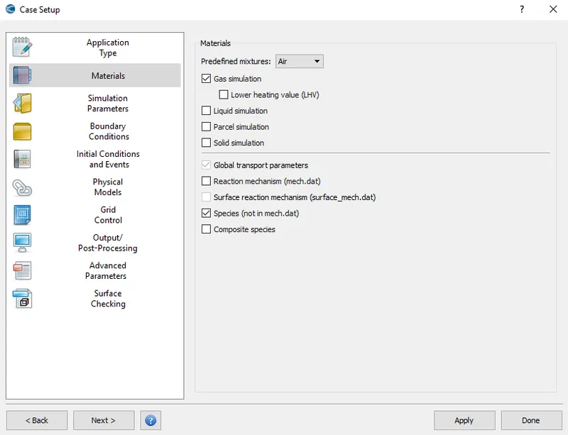
By selecting the predefined Mixture as AIR and checking Species.dat and gas simulation we complete materials setup.
Moving on to another section we have SPECIES where we O2 and N2 in the gas.
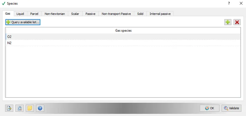
And in SPECIES we have N2 and O2 as the elements which present inside the tube while simulating, From high-pressure zone to low pressure zone.
Moving on to Another section called Run Parameters where we assign very important terms to proceed.
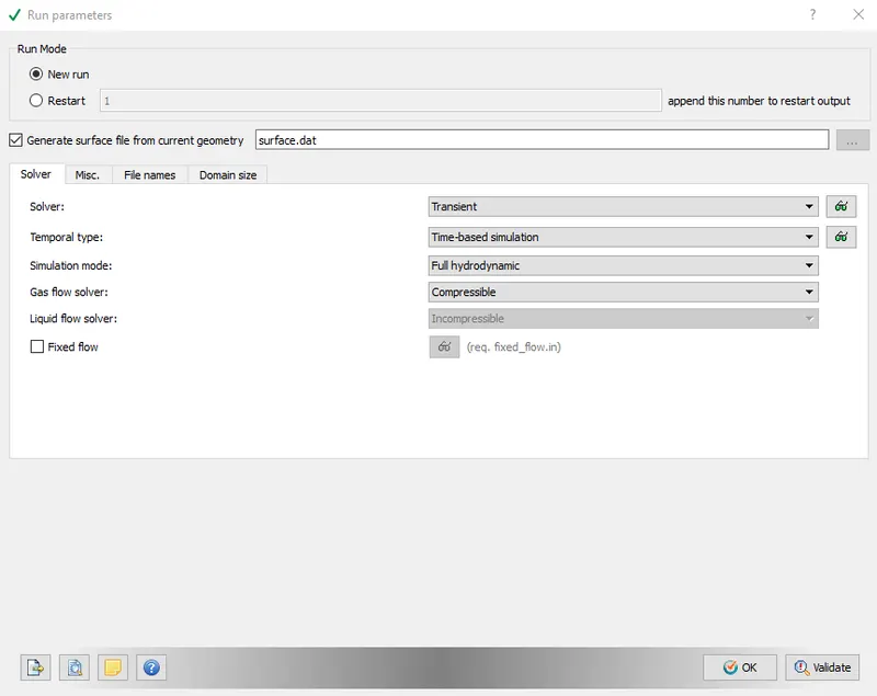
We select Transient solver in the solver section and Full hydrodynamics in the solver section because we are going for simple channel flow. Where there is no complication in this system technically. The full hydrodynamic always take a lot of time to process the data files as it runs the basic Navier stokes equation through and through which might take a lot of time. Hydrodynamics would be a viable option here but again the fluid dynamics properties won't take place while running which is also quite an option in some cases. Since it's a transient flow with Full hydrodynamics option can fully be considered.
Followed by Solver we have the Misc. option where we select the steady-state here again including unchecking the used memory option as we don't want extra storage for the simulation.
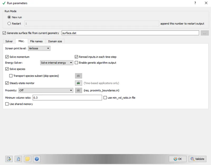
Assigning the value and validating it and Ok.
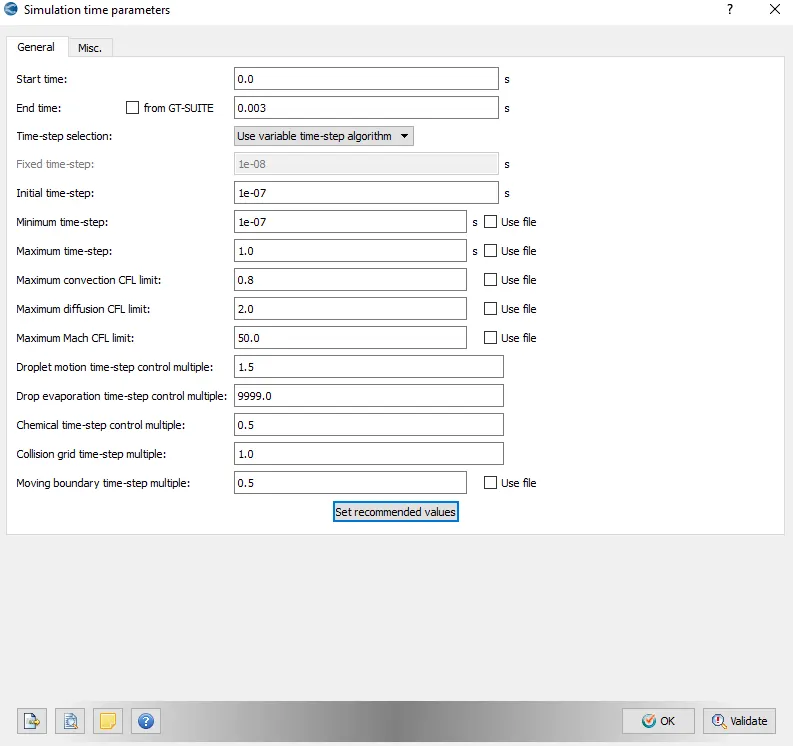
In another section called Simulation-Time Parametres here, we have all the values that are going to be involved in the simulation we are setting up.
The values here as follows for assigning. The end time is 0.003s.
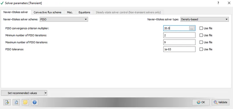
In the nest section of Solver-Parameters, we have what kind type of Navier-stokes solver, which is a Pressure-based solver for this flow.
The next section is really important as we assign the Boundary condition for the flow and the walls around it to define the type of fluid flow effect on it while flowing.
High Pressure - HIGH PRESSURE
Low pressure - LOW PRESSURE
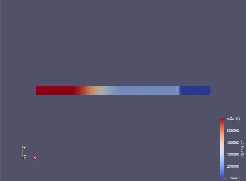
above is how we assign the properties along with section-wise with HIGH PRESSURE 600000.0 Pa and LOW PRESSURE 101325.0 Pa with 300K temperature in temperature boundary conditions.
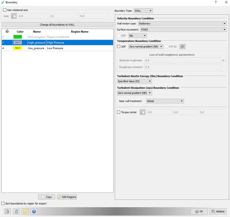
here we have only 2 boundaries which are 3d walls. High-pressure zone and low-pressure zone with a slip boundary wall with fixed and stationary orientation.
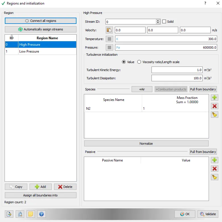
In the Region and Initialization, We need to add the HIGH and LOW-pressure regions which consist of N2 and O2 respectively with a mass fraction of 1.
Now here was have an interesting tool that describes the flow motion of fluid from regions to regions. Its called the EVENTS. we need to put values right like as:
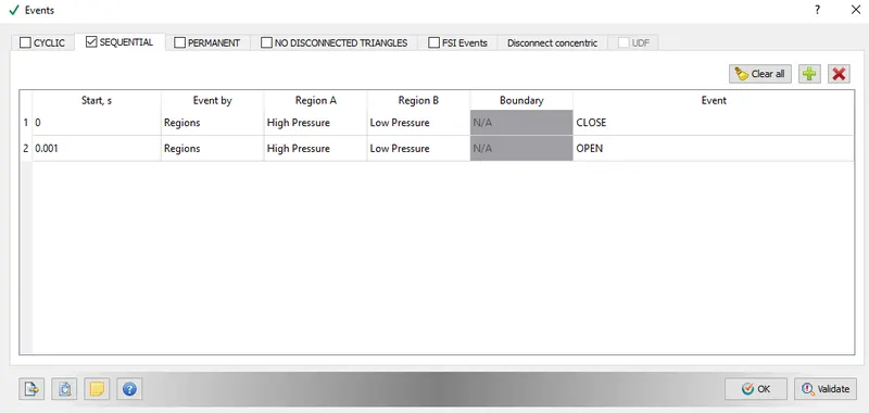
here we commanding the software to CLOSE the regions at 0 and OPEN at 0.001 so the fluid flow can take place from high to low and it gets good motion flowwith regions A and Regions B.
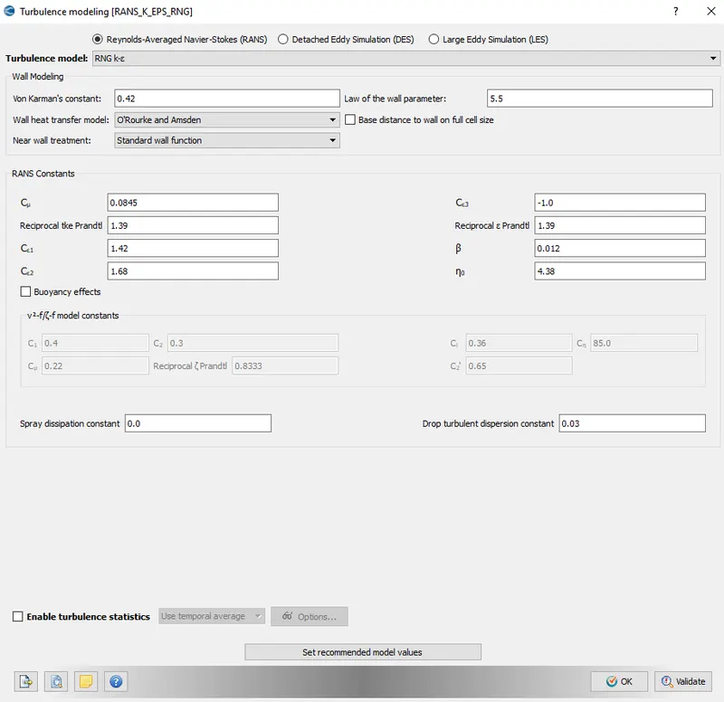
IN the Physical-Modelling We need to check the turbulence modeling as there will be turbulent flow over a channel because of the throttle body. We select the RNG k e method to solve the analysis.
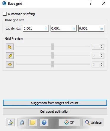
Now the next section is Base Grid, where we assign the INPUT coordinated for the channel so that it has a different output for different inputs. This where the box we create in the first stem gets its own assigned values of coordinates in a cartesian plane.
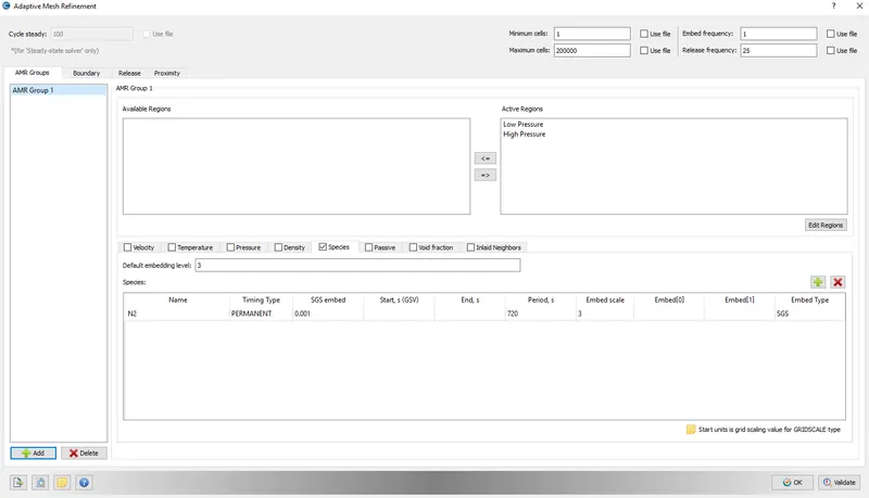
And again we have here AMR Adaptive Mesh Refinement where we are going to give some values so at the shock flow the refinement takes place with mesh looks more clear. And here we pick SPECIES as the variable to mesh refinement with.
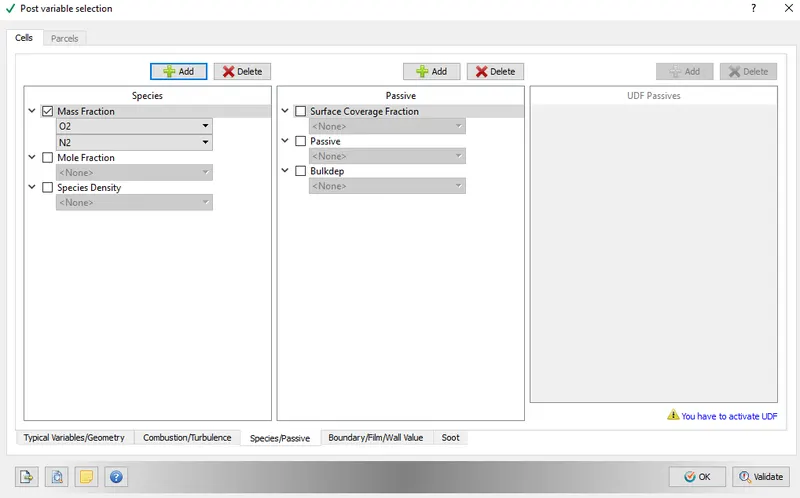
again we have here POST VARIABLE SELECTION where we add N2 and O2 as a Mass fraction.
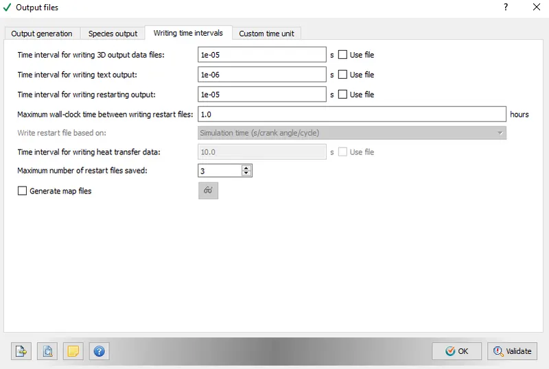
With the SIMULATION oof OUTPUT FILES we have here:
Post-Process Simulation (CYGWIN):
Run Cygwin go to the directory where we have our basic .dat files in the converge folder. These are the following commands in Cygwin to go to the directory
$ cd
and tun the following command to convert,dat files into 3d OUtput dat files.
$ mpiexec.exe -n 2 "" restricted </dev/null> logfile &

This was how-to convert .dat files into 3d Output data files for post-processing.
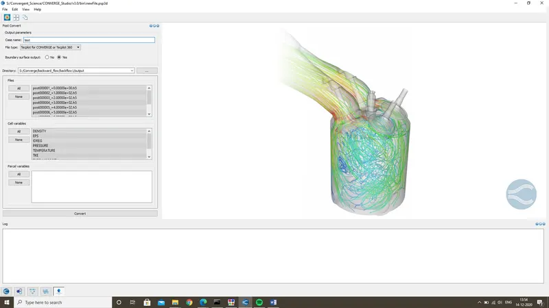
after that, we need to convert those files so that ParaView can read it 3d output files. We need to do through Cygwin to convert those files too with the following command or we can proceed with the converge itself as it provides nice feature to post convert 3D files to DAT files which Paraview can read. Here we need to name it as test and go to the directory of OUTPUT folder where all the files dumped and select ALL and CONVERT just like image shown below. and for post-processing the DAT and files we can directly convert it from CONVERGE as below.
Output:
Pressure Contour and Animation:
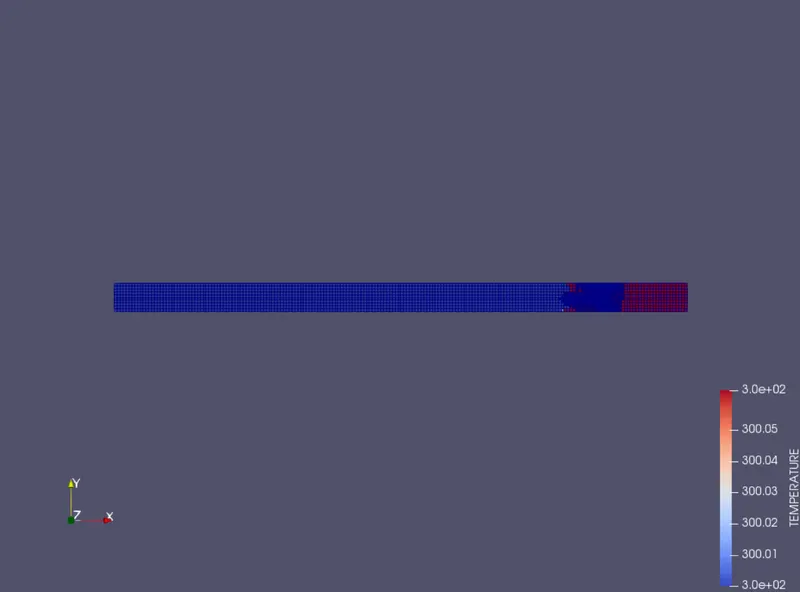
Temperature Contour and Animation:
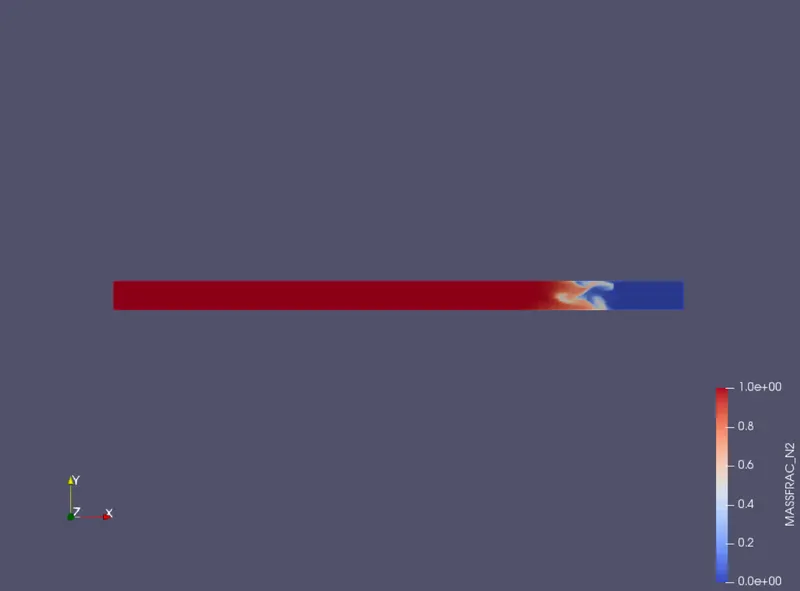
MassFRaction of N2:
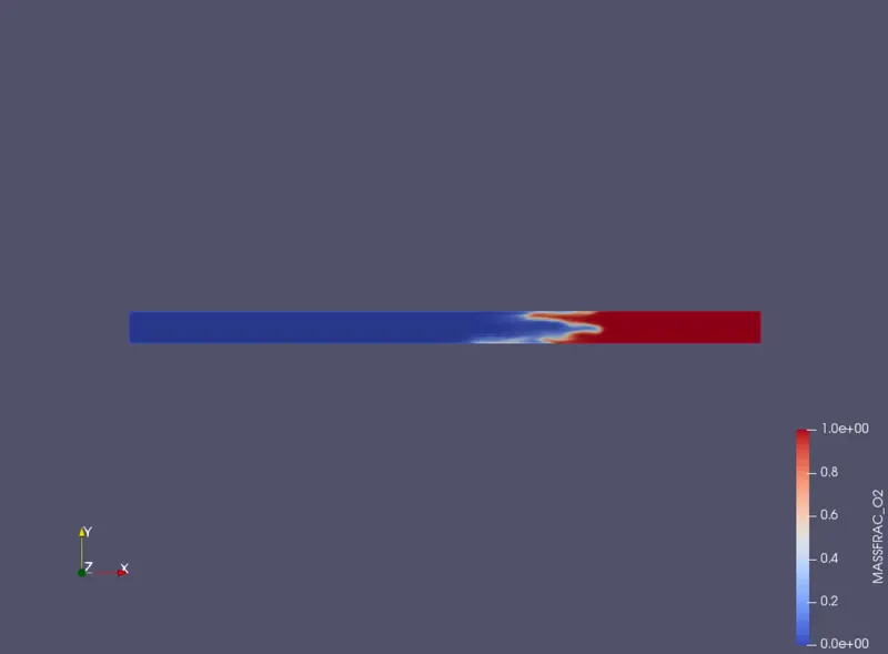
MassFraction of O2 :
Plotting:
We have plot here of Total cell counts, Mass fraction N2, and Mean Pressure from therm.out s both region 0 and region 1:
Total cell counts:
Massfrac of N2:
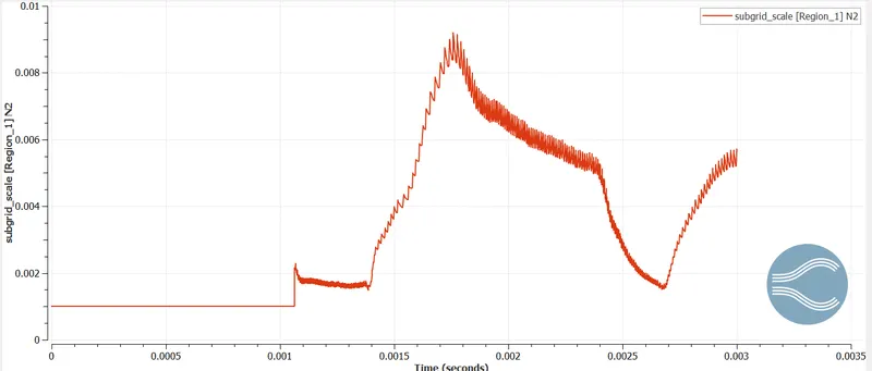
Means pressure at region 0 and 1:
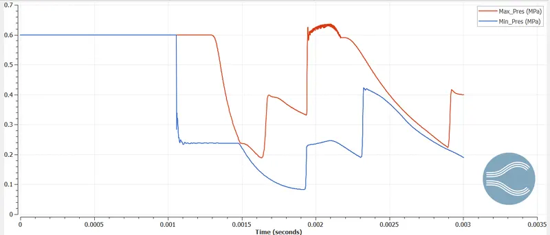
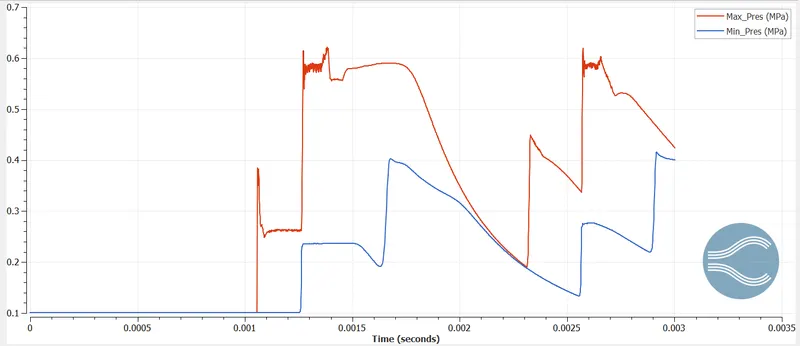
Conclusion:
The Importance of EVENTS in converge is really important as there is a need to connect to disconnect the parts or geometry at a particular time during the simulation. Which can once or multiple times with closing and opening the regions and making the flow over from one place to another omake Autoignition data compared with experimental data.
References:
https://www.sciencedirect.com/topics/physics-and-astronomy/shock-tubes