Week 7: Shock tube simulation project

Aim

To simulate a case of shock tube using converge CFD and study the pressure and temperature characteristics

1. Introduction

A shock tube is an instrument wherein shock waves are generated. The shock wave is produced inside a shock tube when the diaphragm separating a high pressure region (driver medium) and a lower region pressure (driven medium) is broken. A simple shock tube is a tube, rectangular or circular in cross-section, usually constructed of metal

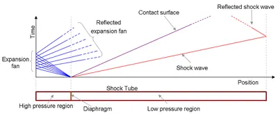
The plot shows different waves which are formed in the tube once the diaphragm is ruptured. At the interface of the two regions, a shock wave is generated due to the pressure difference and propagates towards the driven region. Due to this, the temperature and pressure of the driven medium increases rapidly and a flow with velocity less than the lead wave is imparted into the medium. At the other end, due to the shock generation, a Prandtl-Meyer expansion fan is observed with the Mach lines intersecting at the interface of the two regions.

As the shock waves reach the walls of the low pressure region, the waves are reflected back towards the high pressure region. These reflected waves lead to turbulence and recirculation as they interact with the pressure waves induced in the driven medium. The shock waves are diffused after several back and forth movement and we observe a steady state characteristics for the pressure and temperature inside the shock tube.

The diaphragm suddenly bursts open under predetermined conditions to produce a wave propagating through the low pressure section. The shock that eventually forms increases the temperature and pressure of the test gas and induces a flow in the direction of the shock wave.

1.1 Application

Shock tube finds its application in several domains such as:

• Measurements of rates of chemical kinetics
• fluid flow in the driven gas used as a wind tunnel
• high temperature hypersonic flowused to simulate atmospheric re-entry of spacecraft or hypersonic craft,

Shock tubes can be used to experimentally determine which materials and designs would be best suited to the job of attenuating ambient blast waves

2. Objective

The following are the objectives of the simulation study:

• Setup a transient shock tube simulation
• Plot the pressure and temperature history in the entire domain - Explain the result
• Plot the cell count as a function of time - Explain the result

3. Geometry and boundary flag

For simulating the shock tube, two rectangular boxes are generated.

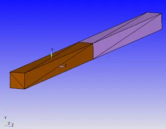
In order to ensure geometry without any interference issues during setting up the event at the interface (discussed in the setup), the interface is constructed with CreateàTriangle

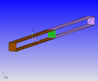
After completing the diagnosis check, the interface of the two regions is deleted.

3.1 Boundary flag

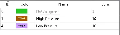
The left rectangular box is flagged as high pressure region and the right box as the low pressure region.

4. Setup

The next step is to setup the case using converge studio.

Application typeà Time-based

Materialsà Predefined mixture- Air & Gas simulation

Run parametersà Solver: Transient

Simulation time parametersà 0 to 0.003 s; Time step : 1e-9 to 1 second ; Max. CFL for convection =1.0

Equations: The max. iterations for energy and pressure solvers are determined based on the simulation warnings

Boundary conditions:

Boundary	Type	Property	Value
High Pressure	Wall	Surface movement	Fixed- Slip
Low Pressure	Wall	Surface movement	Fixed- Slip

Initial conditions and Eventsà Select Events

Region creationà High pressure: 6 bar, Species- N2 (Mass fraction=1)

Low pressure: 1 bar, Species- O2 (Mass fraction =1)

Physical modelà RNG k-Ɛ turbulence model

Grid controlà Adaptive mesh refinement

Base grid: Grid size = 1 mm

Adaptive mesh refinementà Active regions: High pressure, Low pressure

Species- N2, Max cells- 2 Lakhs, Embed scale- 3

Post variable selectionà SpeciesàN2 Mole fraction

Output filesàWriting time intervalsàOutput 3D files: 1e-5 s, text output: 1e-06 s

5. Results and discussion

5.1 Mesh

The above animation shows the surface with edges over the course of simulation. It can be observed that the mesh undergoes refinement based on concentration of N2 gas.

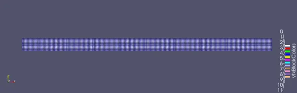
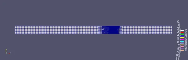
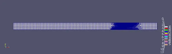
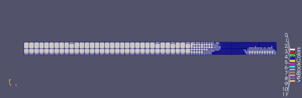
The pattern of mesh refinement can be understood using the animation of N2 concentration as shown below. When the diaphragm is broken, due to the pressure difference, the N2 gas is pushed into the O2 region (low pressure region). This results in compression of O2 gas up to a certain limit. As the given simulation does not consider species reaction, the N2 gas and O2 gas undergo displacement to attain equilibrium and the mesh refinement occurs when there is interaction of compressed N2 and O2 gases.

5.2 Total Cell count

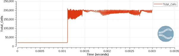
Due to the adaptive mesh refinement, the total cell count changes continuously over the course of simulation

5.3 Velocity

When the diaphragm is broken, the shock waves generated at the interface move towards the low pressure region. This imparts velocity to the fluid medium and we can observe fluid flow from the interface towards the right side. As the velocity reaches the walls, it undergoes reflection and the fluid flow occurs towards other end of the tube. The velocity magnitude drops with successive reflections on the walls of the tube and the fluid flows slowly attains a steady state of rest.

5.4 Pressure

At the interface, when the diaphragm is broken, shock waves are generated towards the low pressure region and the pressure increases as we move the right end of the shock tube. On the other side, the Prantl Meyer expansion fan is generated, originating from the interface moving towards the left wall of the tube. This results in pressure drop (velocity increases). The shock waves after reflecting on the walls of the driven medium start to move towards the driver medium. After multiple oscillations, the pressure inside the shock attains a steady state value.

5.5 Temperature

In constant volume shock tube, the temperature of the gas is directly proportional to the pressure magnitude. After the diaphragm is broken, the pressure of the driven medium increases and consequently, there is a significant rise in temperature. Similarly, the pressure drop on the driver side results in temperature drop to very low magnitude. As the pressure oscillations subside, the temperature attains a steady state. However, on the driven medium, close to the walls, the temperature gradient is observed due to the compression of the gas species.

6. Conclusion

Thus, the case of shock tube was simulated successfully.