Shock tube simulation project

Shock Tube Simulation Using Converge

Aim: To perform a transient simulation of shock tube in Converge.

Objective:

• To setup and perform transient simulation of shock tube.
• To generate pressure and temperatures contours for the obtained result.
• To plot cell cout as a function of time.

Description:

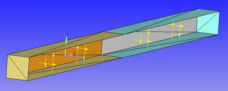
The shock tub is a device in which a normal shock wave is produced by the sudden bursting of a diaphragm seperating a gas at higher pressure from one at lower pressure. Primary use of the shock tube is to study the chemical kinematics. Shock tubes are used in the study of aerodynamic flow under a wide range of temperatures and pressures.A shock wave inside a shock tube may be generated by a small explosion or by the build up of high pressure which cause diaphragm to burs and a shockwave to propagate down the shocktube. It is generally a rectangular or circular in cross-section and usually constructed of metalin which a gas at low pressure and gas at high pressure are seperated using a form of diaphragm. Here, the low-pressure gas is known as the driven gas which is subjectd to shock wave and high pressure gas is called as driver gas. The corresponding sections of the tube are bascially called as the driver and driven sections.

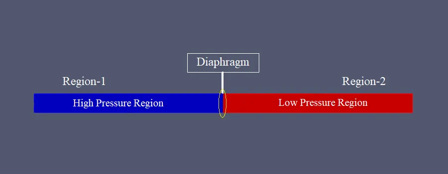
Procedure:

• Initially open Converge Studio and create the geometry or import the geometry which is already created.

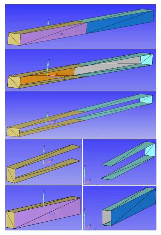
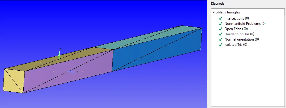
• After setting the geometry, next important thing is to diagnosis the geometry for errors/problems. For this go to Right Bottom side, select Diagnosis > click on All intersections > click Find. On top we can check for problems in Problem Triangles.
• Now if there are no errors found then the geometry is correct.

• So we should do Case Setup. Just beside Diagonisis > click on Cae Setup > in case setup window we can see 'Begin Case Setup" > click on it to set the setup.

Case Setup-

Application Type:

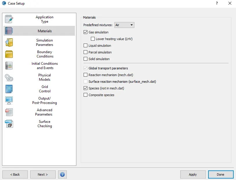
Materials:

Gas simulation

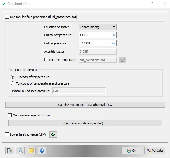
Global Transport Parameters

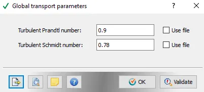
Species

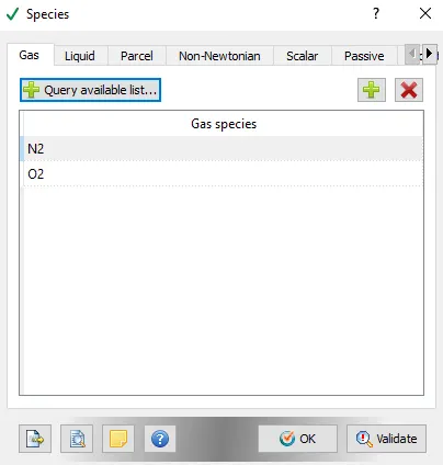
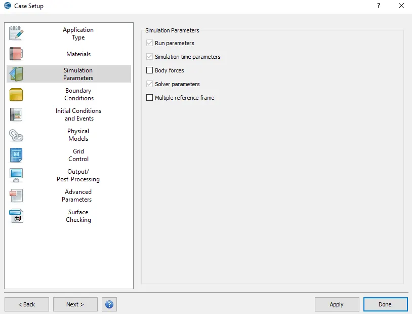
Simulation Parameters:

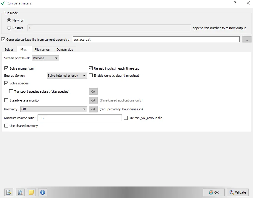
Run parameters

Simulation Time Parameters

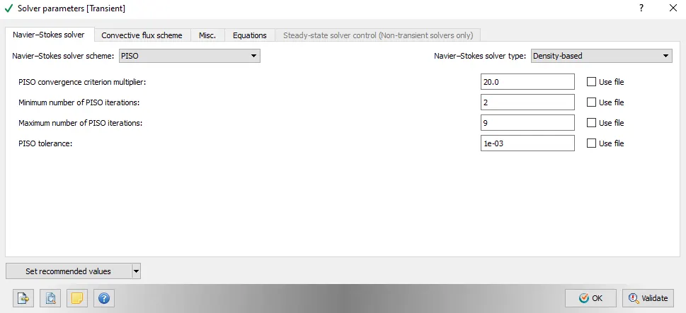
Solver Parameters(transient)

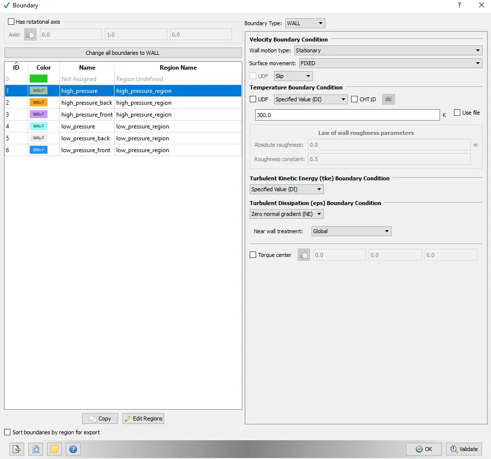
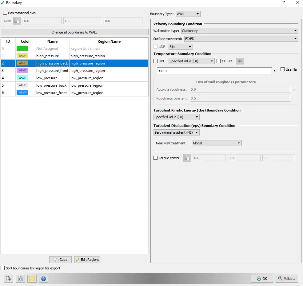
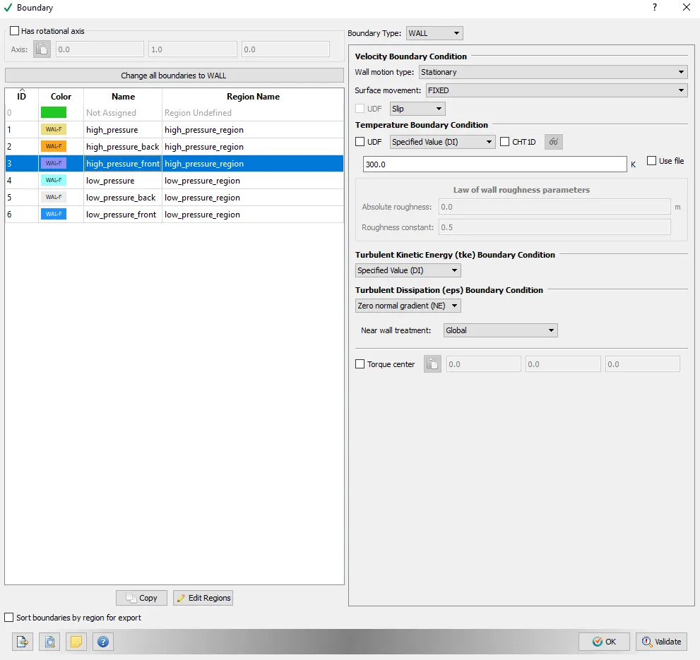
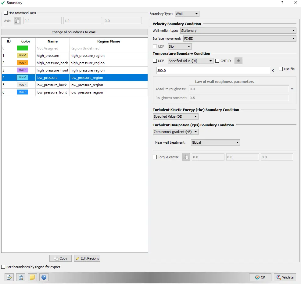
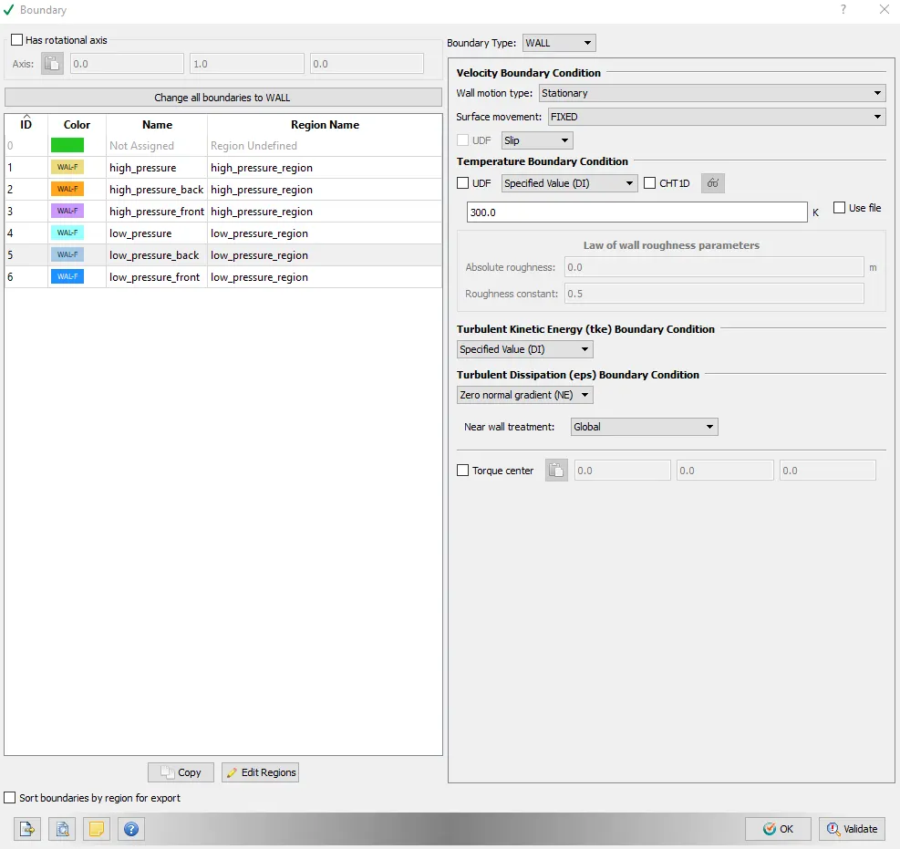
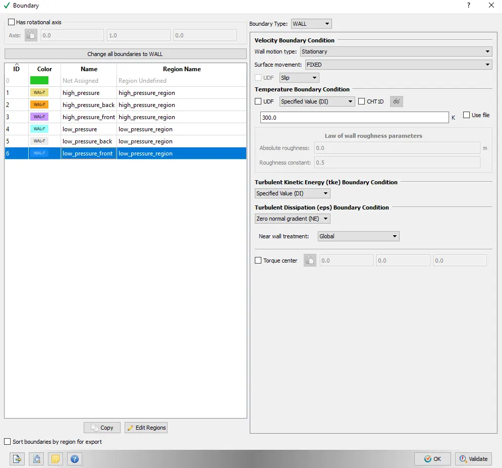
Boundary Conditions:

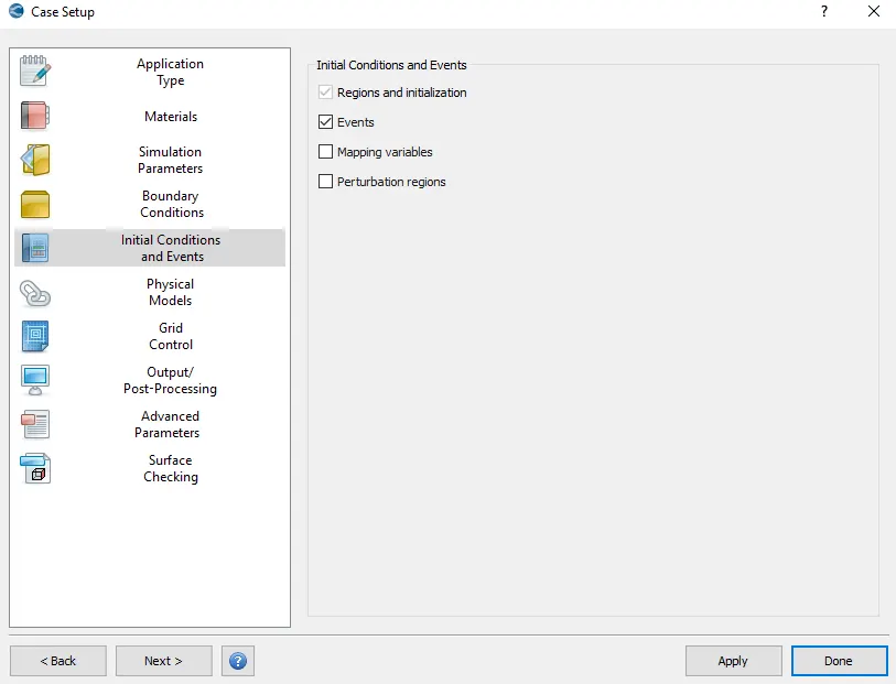
Initial Conditions and Events:

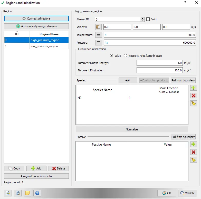
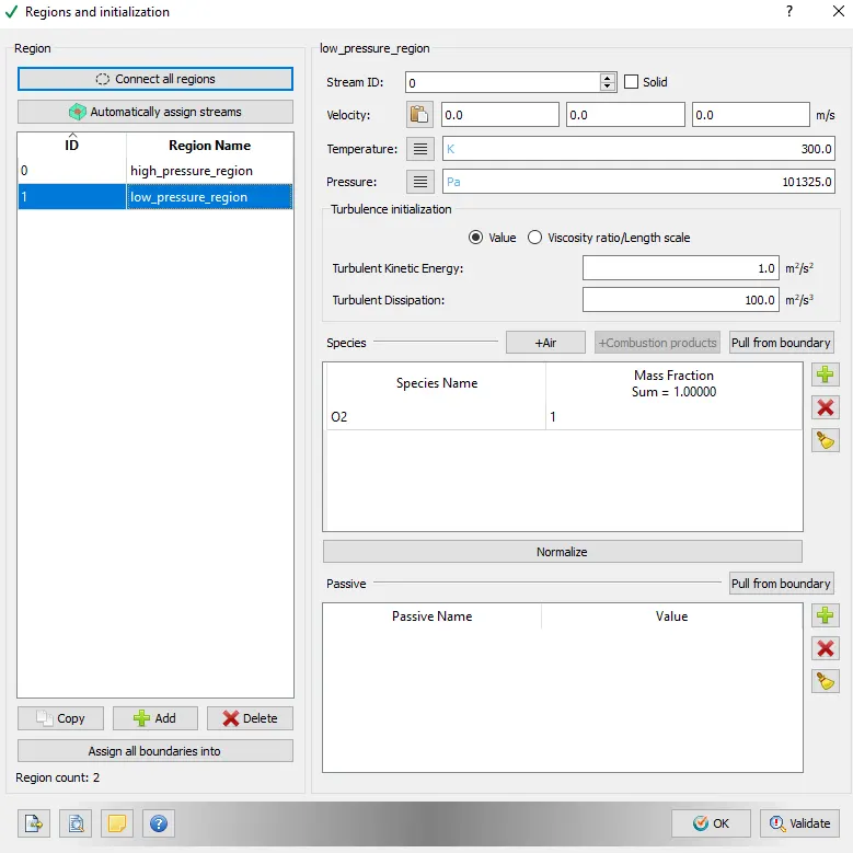
Regions and Initialization

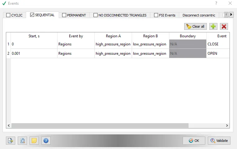
Events

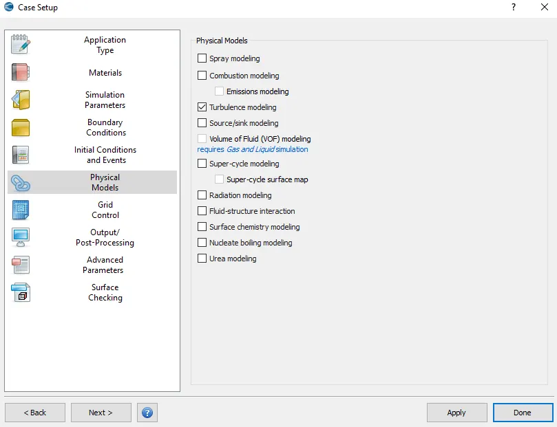
Physical Models:

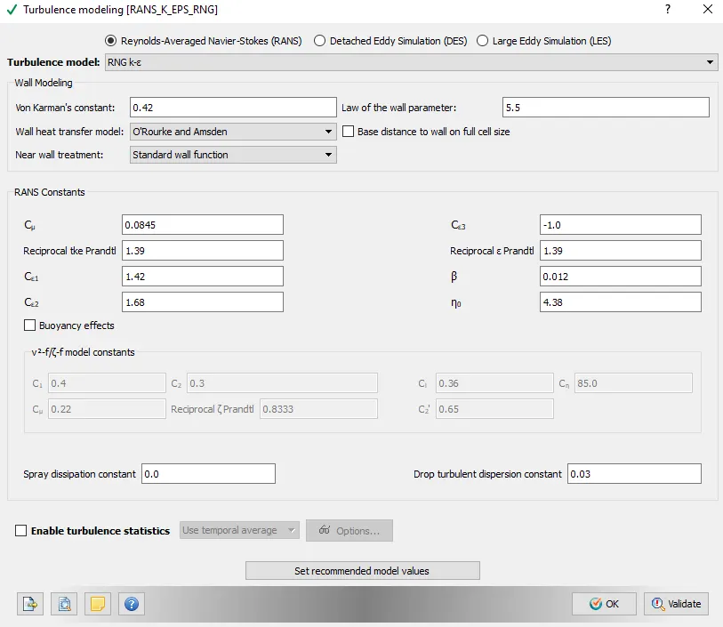
Turbulence Modeling

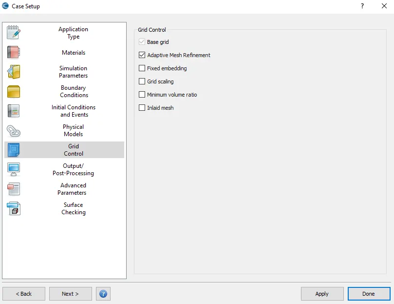
Grid Control:

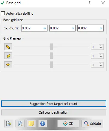
Base Grid

Adaptive Mesh Refinement

Output/Post-processing:

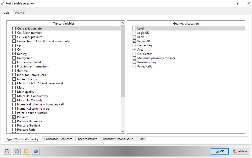
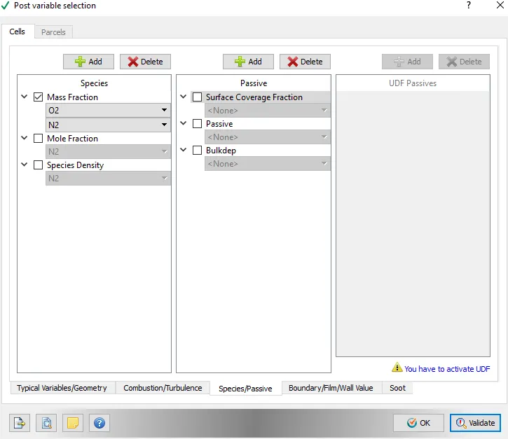
Post variable selection

Click on Typical Variables/Geometry > Select required variables.

Output files

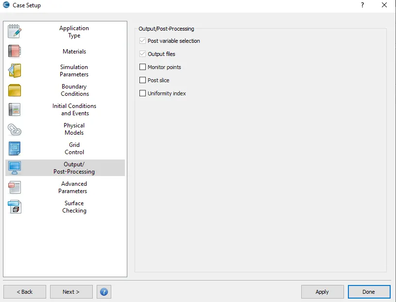
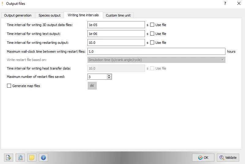
• With this setting up of the case is completed.
• Now go to File > Export > click on Export Input Files. select the destination folder(test) to save the data.

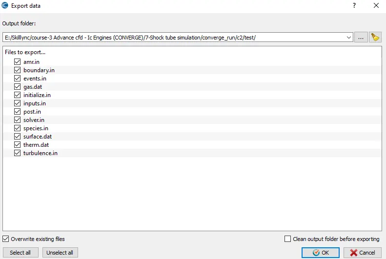
• After importing the input files, paste the "mpiexec.exe file".

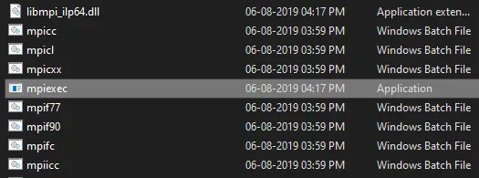
• Now open Cygwin and navigate to the location where the setup files are imported.

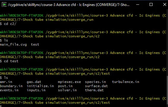
• Once we navigate to the respective folder, we need to run the simulation. To run the simulation, use the following command in Cygwin;

Here path is copied from " C:ProgramFilesConvergent_ScienceCONVERGE3.0.15binconverge-intelmpi.exe ".

• Now the simulation starts running, and it displays the steps in cygwin. As the simulation begins it creates multiple folders (i.e. '.scratch' & output) in the path where we saved the input files.

• Once the simulation is complete, to perform post processing we need to convert the obtained result data into format where we can access in Paraview. These converted files are directed to the Output folder.

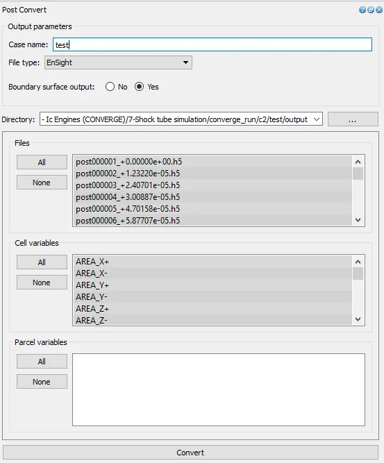
• Open PARAVIEW > direct to folder where the output is saved > select '.vtm(group file) or .case file' > data imported to paraview.

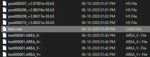
• Necessary contours, profiles and animations are generated using paraview. To generate plots we can use ConvergeStudio (line plotting option).
• Hence required plots, contours, animations are obtained in order to study the results.

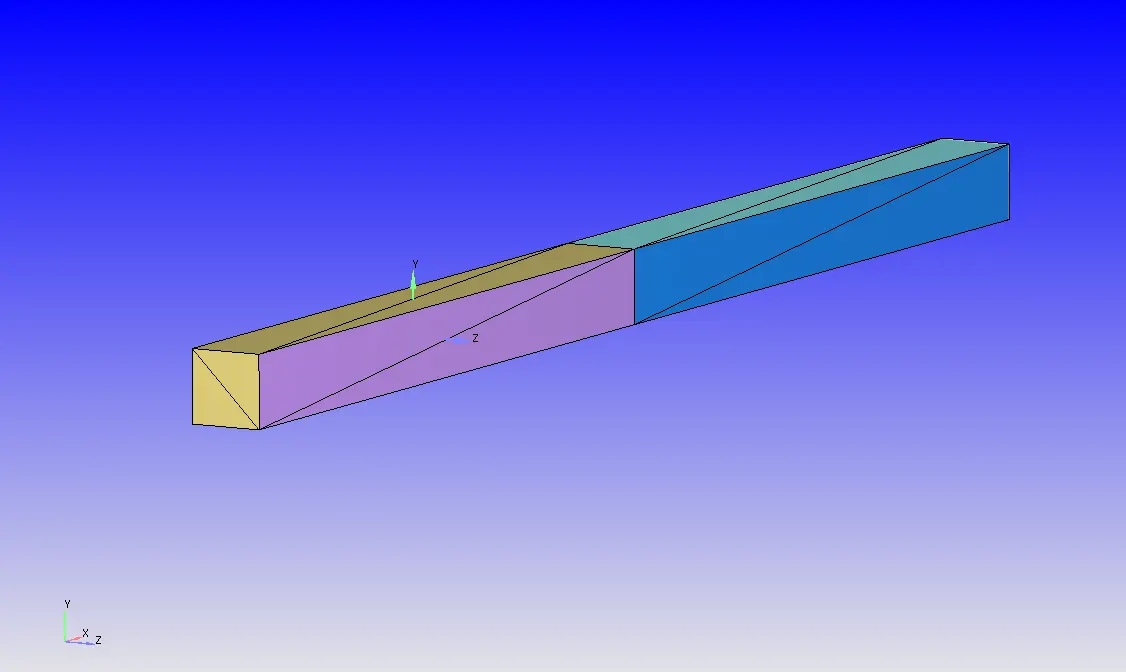
Geometry:

Observations:

Mesh:

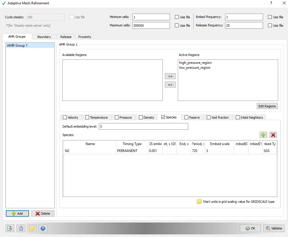
Adaptive Mesh Refinement:

AMR mesh generation contour:

Pressure Contour:

Temperature Contour:

Velocity Contour:

Mean Temperature plot:

Pressure plot:

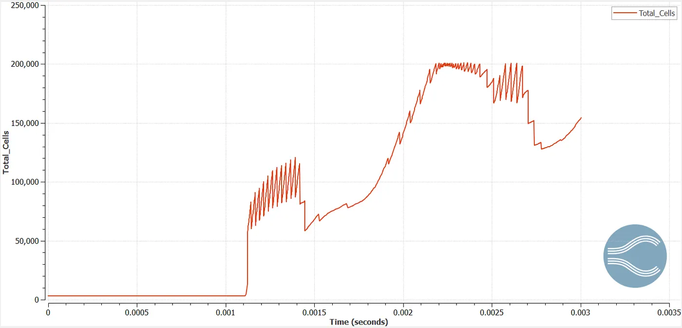
Cellcount (grid size=0.002m):

Animations:

Temperature-

Pressure-

Velocity-

Mass Fraction of N2-

Mass Fraction of O2-

Results:

• From the cell count plot it is observed that from 0 seconds-0.001 seconds, the diaphragram is closed. Once the 0.001second is over the diaphragram is broken. When it is broken with the flow Adaptive Mesh Refinement(AMR) gets active. Hence after that point we can observe that high pressure intract with low pressure. Because of this there is sudden increase in cell count.
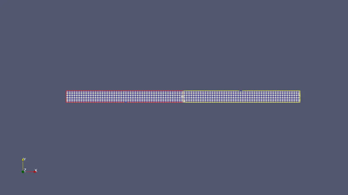
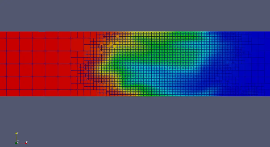
• From the generated mesh profile (AMR), we can see that it has embeded the mesh size by 3 levels with the SGS value of 0.001. This kind of refinement elps to capture good characteristics of the gas flow through the domain, importantly captures the propagation of the reflected shock waves and gives better understanding of chemical kinetics.
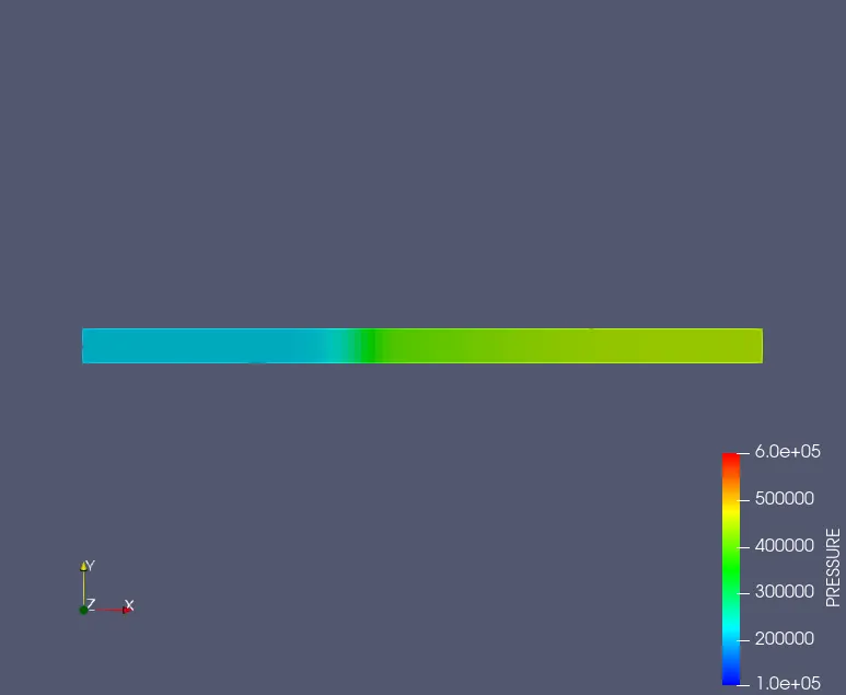
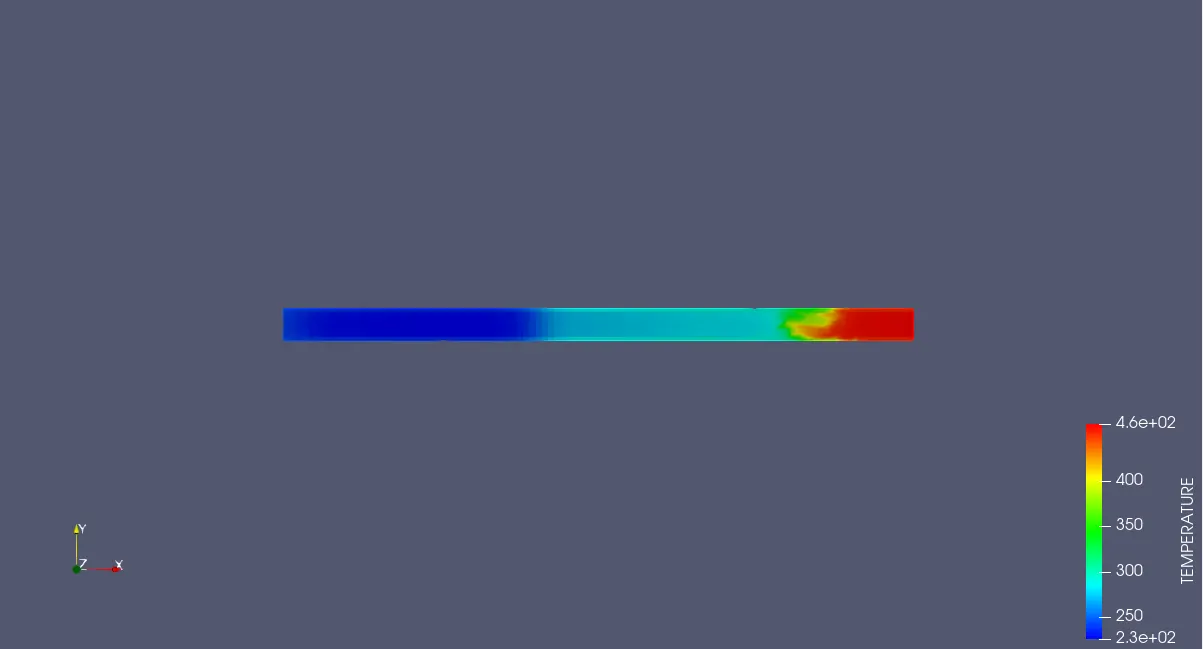
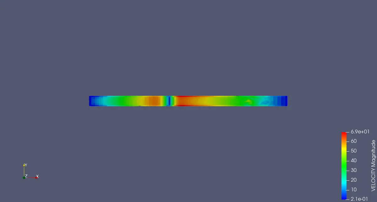
• The contours generated represent the variation of properties through the simulation.The provided animations clearly shows how the diaphragm breaks and due to the pressure difference the shock waves are developed and gradually these waves reflect from the walls and get refraction waves.
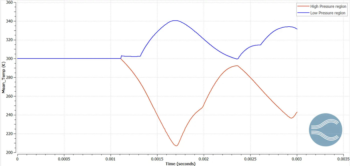
• The driven gas undergoes compression and expansion by variations in pressure and temperature. Hence the driven gas reflects back in the form of reflected waves i.e. shock wave. Due to compression, the pressure in the driven region increases by the expansion of high pressure gas, the temperature increases. When the pressure in the driven section decreases due to the expansion of the driven gas, the temperature in the section decreasses.
• As the diaphragram breaks at particular point, the gas from high pressure region flows into the low pressure region. So the temperature plot clearly shows that the temperature is decreased for the high pressure region and increased for the low pressure region.
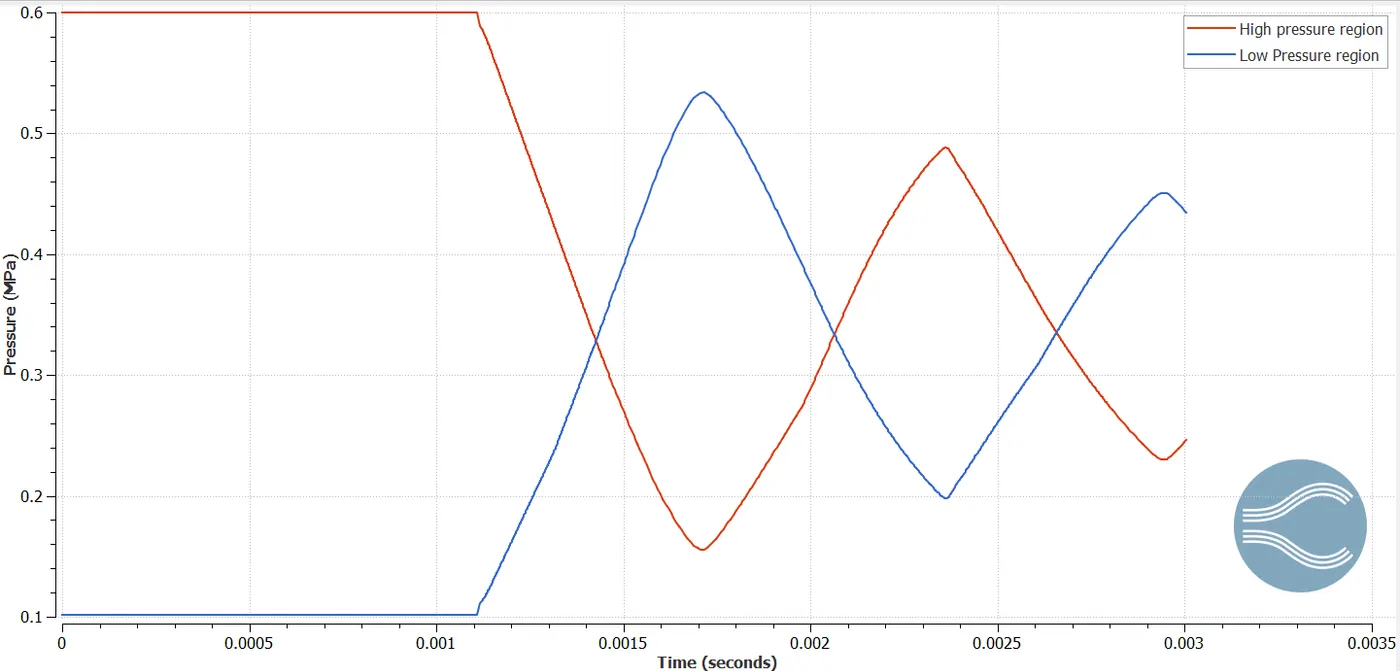
• Considering the pressure plot, for higher pressure region the initial pressure is taken as 6bar and for the low pressure region it is taken as 1bar. When tha diaphragm breaks and both the regions interact and form the profile that is shown above.
• The species(O2,N2) concentration is also generated to understand their behaviour during the flow.

Conclusion:

A transient shock tube simulation is performed in order to study how the fluid flow effects in the shock tube. Adaptive Mesh Refinement is included during the simulation as it helps to understand the flow more clearly.For better and accurate results the finely refined mesh case is considered. Various plots , contours and animations are generated to understand the chemical kinetics in a shock tube.