Week 7: Shock tube simulation project

SHOCK TUBE SIMULATION WEEK -7

A shock tube is simple but a really impot tool for studying various things under fluctuating temperature and pressure. Various application where shock tubes are used :

• replicate and direct blast waves at a sensor or a model to simulate actual explosions effects.

• to study aerodynamic flow under a range of temperatures and pressures difficult to obtain otherwise.

• to study compressible flow phenomena and gas phase combustion reactions

• in biomedical research to study how biological specimens are affected by blast waves.

• to measurements of rates of chemical kinetics, dissociation energies and molecular relaxation rates.

“A shock wave inside a shock tube may be generated by a small explosion (blast-driven) or by the buildup of high pressures which cause diaphragm(s) to burst and a shock wave to propagate down the shock tube (compressed-gas driven)”.[2]

A simple shock tube may be circular (or rectangular ) in cross-section. It's usually constructed of metal, in which a gas at low pressure and a gas at high pressure are separated using diaphragm. Diaphragm suddenly bursts open under predetermined conditions to produce a wave propagating through the low pressure section. The shock formed increases the temperature and pressure of gas. It also induces flow in the direction of the shock wave.

The LP gas, referred to as the driven gas, while HP gas is known as the driver gas. The LP gas is subjected to the shock wave. The corresponding sections of the tube are correspondingly called as driver and driven sections.

To obtain the strongest shocks the pressure of the driven gas is well below atmospheric pressure.

Shock tubes have been developed in a wide range of sizes. The size and method of producing the shock wave determine the peak and duration of the pressure wave it produces.

The Video is Available here.

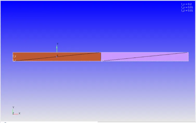
Domain:

Mesh:

Key Setup Points:

Simulation type : Transient

Start time: 0 sec

End Time : 0.003 sec

Base grid : 0.001mm

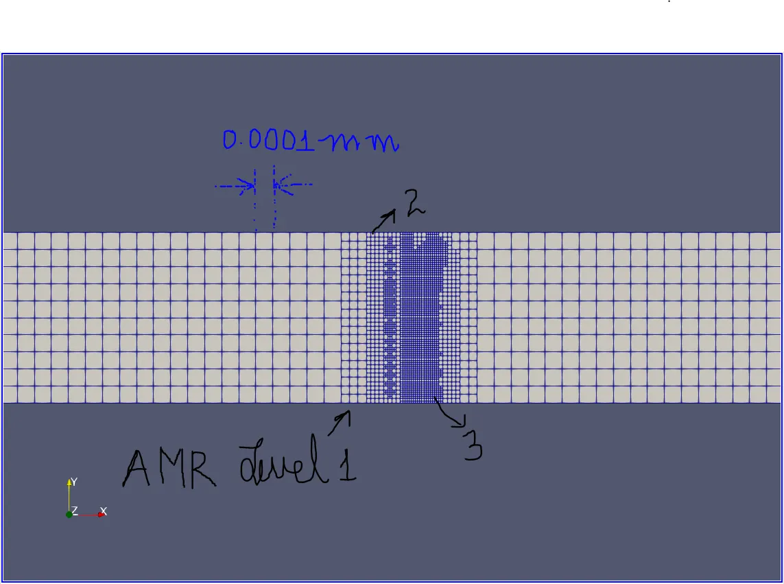
AMR Flag: 1

AMR level: 3

AMR Base: Species (For O2)

Boundary :

• High Pressure Side; Specie: O2; Pressure: 6 Bar

• Low Pressure Side; Specie: N2; Pressure: 1 Bar

Event Flag: 1

• Sequential between HP and LP regions

• Close up to 0.001 sec

• Open After 0.001 sec

Species:

• O2 in HP region

• N2 in LP region

RESULTS:

Temperature vs Time:

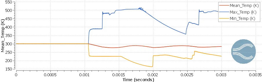
• It’s evident from the graph that as the HP region is allowed to expand into the LP region there is fluctuation of temperature in the domain.

• This fluctuation is quite as expected.

• It's a characteristic feature of shock wave formation and hence is also an indicator that the shock must have formed in the domain.

Pressure vs Time

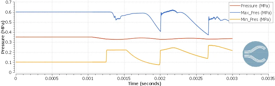
• Above figure shows the pressure variation in the domain with time.

• Here also as the HP region is allowed to expand into the LP region there is fluctuation of pressure in the domain.

• This fluctuation is quite as expected.

• It's a characteristic feature of shock wave formation and hence is also an indicator that the shock must have formed in the domain.

• Mean domain pressure has merely any change.

Total Cell Count vs Time:

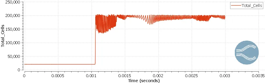
• AMR is active and is based on species.

• As the interaction between species starts soon after sec the amr comes into picture.

• We can see clearly that amr kicked in just before 0.0011 sec which definitely shows that it takes a while to reach the SGS cutoff value.

• The maximum number of cells is set to 200000 and here the cell count lies hover around it.

This is not that interesting, well What is is shown below:

Region Pressure variation with time:

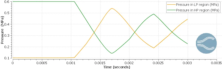
• One can easily make out the wavy nature of the plot suggesting the formation of shock waves.

• As the HP expands into the LP region there is a pressure drop in HP while a rise in LP.

• This exchange goes on but there is a catch here.

• The peak's value goes on decreasing as the system tries to attain stability.

• If the simulation is done for sufficient time one can see the stabilized pressure of the system.

Region Temperature variation with Time:

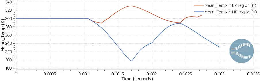
• The temperature of the LP region decreases a bit as the two regions open but then starts to increase as HP expands into LP.

• This is purely because compression of gas causes its temperature to increase.

• Similarly, expansion of other causes its temperature to decrease.

• One can also see that increase in LP temperature is not reflected proportionally by decrease in HP temperature.

• Also there is interaction of energy from one form to another which may be the reason for the above observation.

References:

• Google Search.

• Wikipedia.

• Book on Numerical Analysis for Fluid and Heat Transfer Problems.