Week 7 - Mini project - Flow over an Airfoil

Introduction

The objective of the current study is to simulate the flow of air over a standard NACA 2412 airfoil. Simulations are carried out for different angles of attack to study the effect of the inclination of the airfoil on the drag and lift coefficients.

An airfoil refers to the cross-section area of an aerodynamic body that is subjected to different aerodynamic forces, depending upon its geometry and orientation. The most common example of an airfoil is the cross-section area of the wing of an aircraft. The aerodynamic forces acting on the airfoil are responsible for allowing the aircraft to take off from the ground.

The two primary aerodynamic forces acting on an airfoil are Drag and Lift. The drag force acts parallel to the flow of the fluid and tends to oppose the forward motion of the airfoil. The lift force acts perpendicular to the drag force and tends to lift the airfoil upwards. Aircrafts are designed to minimise Drag and maximise Lift. The drag and lift forces are calculated by the formulae mentioned below:

Fd=2Cd/(ρ⋅V⋅A)_________________________________i

Fl=2Cl/(ρ⋅V⋅A)_________________________________ii

where Fd= Drag Force (N)

Fl= Lift Force (N)

Cd= Drag Coeffiecient

Cn= Lift Coeffiecient

ρ= Density of the fluid (kg/m3)

V= Free-stream velocity of fluid (m/s)

A= Acting area of fluid (m2)

An airfoil generates lift by the use of Bernoulli's principle. According to the Bernoulli's Principle, for a fluid moving around a body at different velocities, the fluid exerts a higher pressure on the body for a lower velocity than it does at a higher velocity. The curved shape of the airfoil causes a significant jump in velocity of the air around the upper surface of the airfoil, while there is a significant reduction in the velocity across the lower surface of the airfoil, mainly due to the geometry of the airfoil and viscous effects. As a result, a higher pressure, perpendicular to the direction of air flow, is exerted on the airfoil on the lower surface while a relatively lower pressure is exerted across its upper surface. This pressure difference leads to the formation of a net force in the upward direction.

Computational Details

The simulations are carried out by using Converge Studio 3.0 as the preprocesser and ParaView 5 as the post-processing tool. A structured mesh with a grid size of 0.08 m is adopted for the current simulation due to computational restrictions. However, to improve the accuracy of the result, Fixed Embedding with 2 layers and at a scale of 2 is adopted.

Initial simulations were carried out at steady state. Due to inaccurate results and a lack of convergence, transient simulations were chosen. The required boundary conditions suggest an inlet Reynolds number of 2,00,000.

Re= ρ.V.C/μ_________________________________iii

where Re= Reynolds Number (2,00,000)

ρ= Density of air (1.2 kg/m3)

V= free stream velocity

C=chord length (0.1 m)

μ= Dynamic viscosity (1.81 x 10^(-5) Pa.s)

The above values give a free-stream velocity of ~30 m/s.

The airfoil dimensions were scaled down by a factor of 0.1 to reduce computational load. Thus, a wind tunnel with a length and height of 5 x 3 m was adopted.

The flow time is calculated to be 5/30= 0.167 s. The total simulation time was taken to be 1.5 s, with a minimum step time of 1e-05 s.

The inlet and outlet boundaries were marked as inflow and outflow boundaries respectively. The airfoil wall was given a WALL boundary condition with law of wall. The upper and lower surfaces of the wind tunnel were marked as symmetry boundary conditions.

Two turbulence models, namely RNG k-ε and k-ω SST were used. The entire region was initialised with a velocity of 30 m/s and a temperature of 300 K.

Results and Discussions

Velocity contour simulations for the k-ω SST model

Angle of attack= 1º

Angle of attack= 5º

Angle of attack= 10º

Angle of attack= 15º

Prelimnary observations suggest that as per the Bernoulli's principle, there is a sudden jump in the velocity of the air as it moves over the upper surface of the airfoil, leading to a lower pressure force on the upper surface and a higher pressure across the bottom surface. As the flow progresses further downstream across the airfoil, there is a reduction in the velocity due to increase in the pressure exerted. There is an evident increase in the low pressure region above the airfoil as the angle of attack is increased, as indicated by the velocity contours. Furthermore, increasing the angle of attack tends to create further obstruction to the flow of air, resulting in a greater drag force. The estimated trend suggests that increasing the angle of attack should lead to greater lift and drag forces.

Variation of Drag Force

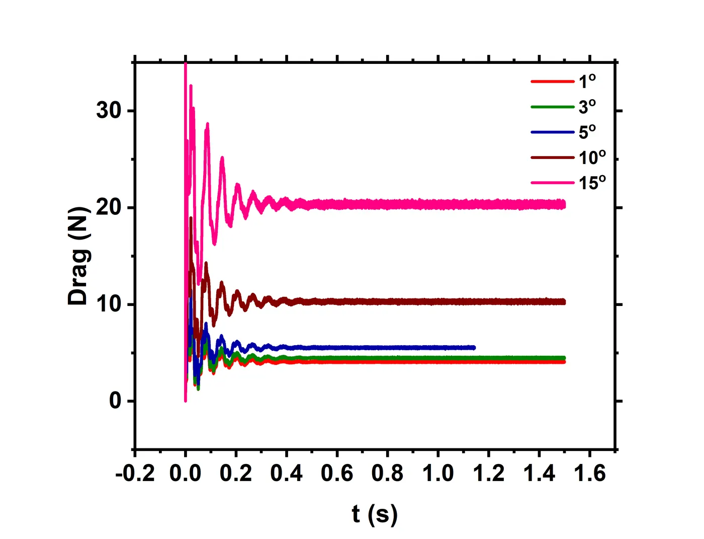
The above graph shows the variation of the drag force with time for different angles of attack. As predicted earlier, there is an increase in the drag force with increasing angles of attack due to the obstruction offered by airfoil to the flow of the air. A maximum drag force of ~20 N is obtained in case of an angle of attack of 15º

Variation of Lift Force

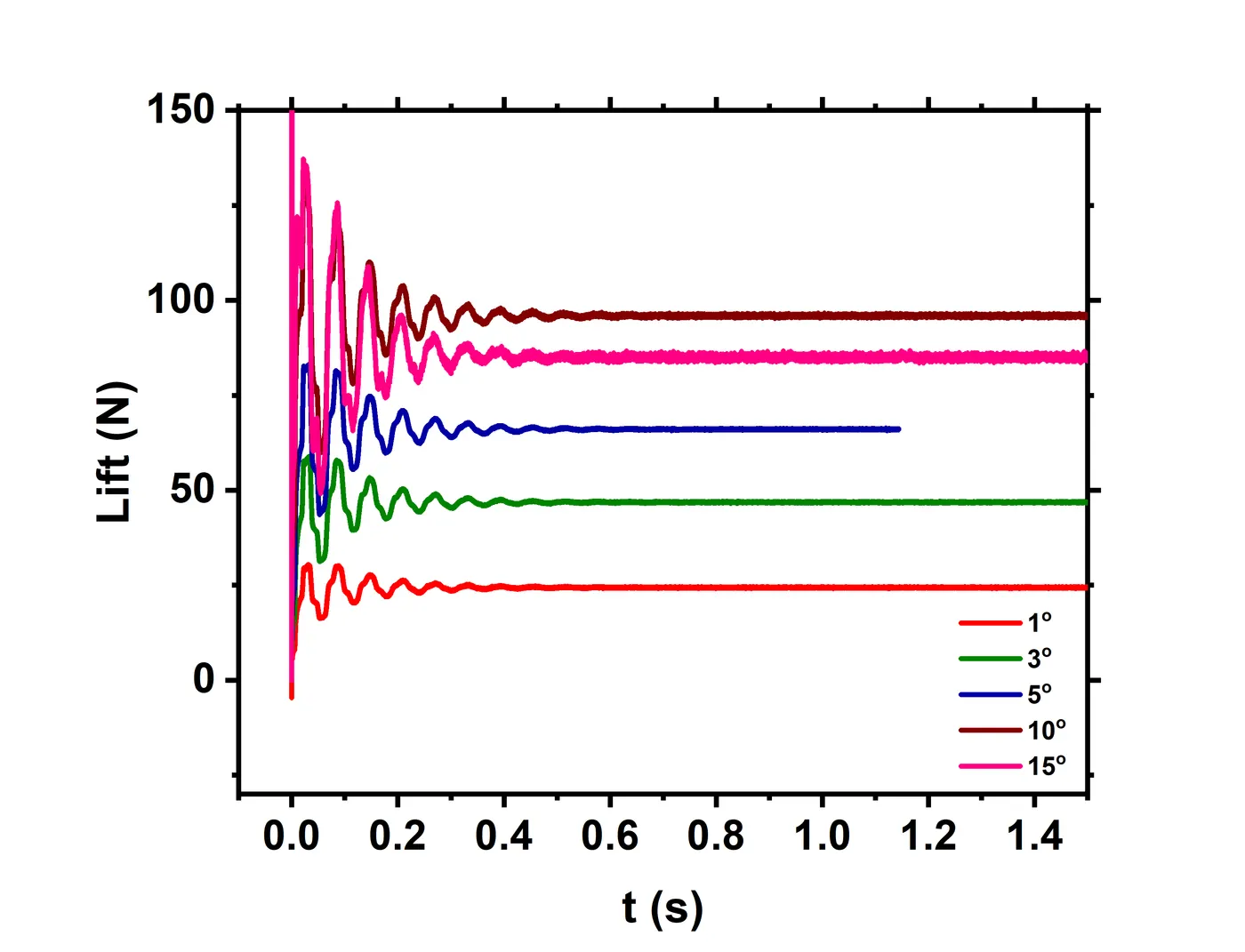
The above figure shows the variation of the lift force with time for different angles of attack. The lift force generated increases with increasing angle of attack upto 10º. The lift force obtained in case of 15º is lower than that obtained in case of 10º, which goes according to the predicted trend. This behaviour is interesting and can be attributed to the flow separation observed in case of the 15º simulation, as is shown in the video above. This leads to a significant reduction in velocity across its trailing edge, leading to the formation of a higher pressure zone than its 10º counterpart.

Effect of Turbulence Models

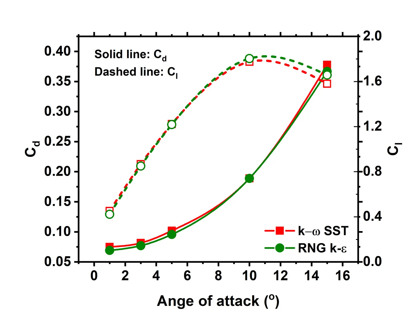
The above simulations have been carried out for the k-ω SST and RNG k-ε turbulence models. The graph plotted below shows the variation of the drag and lift coefficients with angle of attack for both the turbulence models. The results obtained below confirm the readings reported above, indicating that there is a reduction in the lift force generated when the angle of attack is varied from 10º to 15º. It is interesting to note that although there is negligible variation between both models for the drag coefficient, there is tangible deviation between the models in case of the lift coefficient. Since the lift coefficient is significantly impacted by flow separation in the boundary layer, it is crucial to choose the turbulence model that is more accurate closer to the boundary layer.

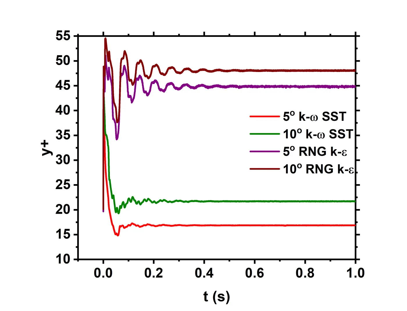
To determine the accuracy of the turbulence models, variation of the normalized distance (y+) parameter with time for both turbulence models and angles of attack 5º and 10º are plotted below. The y+ parameter is a measure of the location in the boundary layer. y+<30 usually indicates the buffer layer. Given that our area of interest lies in the flow separation, that occurs in the buffer and viscous sub-layers, it is desirable to have a low y+. Hence, the k-ω SST model is adopted in the current case.

Conclusion

The results obtained in the above simulations indicate that increasing the angle of attack leads to an increase in the drag force. There is a rise in the lift force until the angle of attack approaches 15º. This is attributed to the flow separation effect that occurs at 15º. Furthermore, the k-ω SST and RNG k-ε turbulence models are compared, with a lower y+ value obtained for the former.