Week-7 Head Impact

Pedestrian Head Impact Test Simulation

Aim: To simulate the impact of a pedestrian headform on a car hood (at three separate points) and calculate the Head Injury Coefficient (HIC) for the collision. The HIC values will then be analyzed to deduce the nature and seriousness of the injury to the pedestrian.

Introduction and Theoretical Background: There are three types of crash or impact tests carried out on commercial automobiles - structural crashworthiness, occupant safety, and pedestrian impact tests. Pedestrian impacts can cause mild to severe injuries and even fatalities. The most serious injuries are caused by full-frontal collisions [1]. The most common injuries are experienced in the head, torso, and limbs with the most serious injuries being noted in the head. The Head injury coefficient computed from a head impact test gives the likelihood of a certain level (of seriousness) of head injury occurring in case of a collision with a pedestrian. Based on the Gadd Severity Index (GSI), the HIC is calculated as:

........................(i)

The value obtained from equation (i) is called Free Motion Headform HIC since it is not connected to a body. As per FMVSS201U, this value is used to compute what is called HIC(d), which gives the value of HIC that would have been obtained from the tests if the head was attached to a body.

HIC(d) = 0.75446*(Free Motion HIC) + 166.4................................(ii)

The time period (t1-t2) should be at least 3ms - below this, there is no risk of injury to the brain- and a maximum of 36ms or 15ms (for HIC36 and HIC15 respectively) - for decelerations above 36ms, there is no increase in risk to injury.

It is important to note that the HIC value does not indicate the level of seriousness of injuries, rather the probability of occurrence of different levels of injury. As per FMVSS201U, HIC36 for commercial automobiles has been limited to 1000 and HIC15 to 700.

Geometrical setup, and spatial discretization: The model was built up in three stages, starting with the simplest impact model and adding complexities in successive stages.

• Case1: For the first simulation, a simple sphere with 979 quad elements, was made to impact against a rigidwall at 45 degrees inclination. The quads were given 5 integration points through thickness and an element formulation of 6 (S/R Hughes Liu). The spherical headform was imported using the *INCLUDE command.

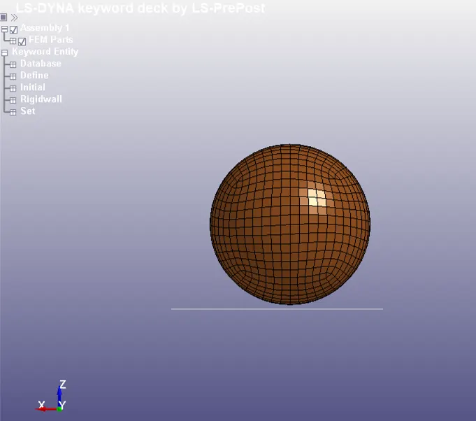
Fig1: Geometrical setup with simple sphere and rigidwall

• Case2: In this case, the sphere was replaced with an actual headform made up of four parts - the skin, skull, accelerometer block, and the backplate. The skin, skull, and backplate were meshed with 20027 hex elements and a seatbelt_accelerometer element model was used for the accelerometer block. The hex elements were left with the default element formulation of 1 (constant stress solid elements). An Hourglass control with IHQ 7 was assigned to it. The Headform was imported using *INCLUDE_TRANSFORM command with a transformation id corresponding to the *DEFINE_TRANSFORMATION card. The transformation involved rotating the headform by an angle of 45 degrees about the Y-axis.

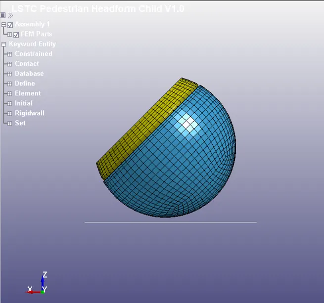
Fig2: Geometrical setup of Actual Headform with rigidwall

• Case3: Here along with the headform model, a meshed hood part with 10373 shell elements (quad dominated) was used instead of the rigidwall. The shell elements were given a formulation of type 7 (S/R co-rotational Hughes Liu). The meshed hood was imported without any transformations but using the *INCLUDE_TRANSFORM and *DEFINE_TRANSFORMATION (just in case any transformations seemed necessary later on). The headform was imported and rotated as in Case2, but for this case, three different impact points were selected to get the HIC values at different locations on the hood. Point one was along the neutral Y-axis, point two was 300mm to the left of point 1, and point 3 was 350mm to the right and 300mm above the point1. The Translate option in Define_transformation was used to orient and position the headform at these locations.

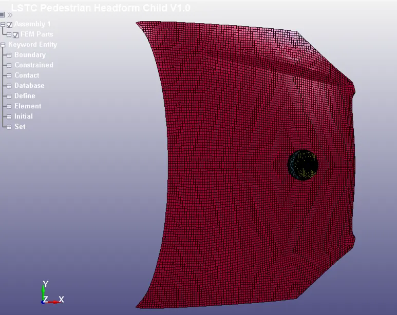
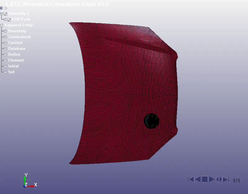
Fig3: Geometrical setup for Impact point 1 Fig4: Geometrical setup for Impact point 2

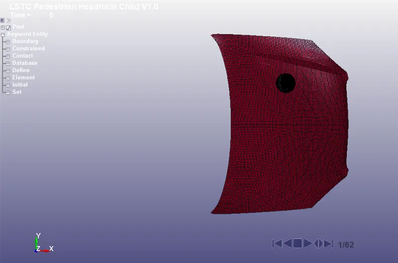
Fig5: Geometrical setup for Impact point 3

Constitutive Material Model: For the spherical headform a simple MAT_Elastic model was used with the following properties:

Sl No	Material Property	Magnitude	Unit
1	Density	3e-06	kg/mm3
2	Young's Modulus	5465e-03	GPa
3	Poisson's Ratio	0.22	-

Table 1: Material properties for elastic headform [3]

For the actual headform, the material properties were included in the imported ls-dyna file and no changes were made to it. The skull, backplate, accelerator block had been provided a MAT_Rigid card and the skin MAT_O_Ogden_Rubber card.

The meshed hood was assigned a Piecewise_linear_plasticity card with the material properties being modelled along the lines of a 6000 series aluminium alloy.

Sl No	Material Property	Magnitude	Unit
1	Density	2.87e-06	kg/mm3
2	Young's Modulus	70	GPa
3	Poisson's Ratio	0.3	-
4	Yield Stress	0.24	GPa
5	Tangent Modulus	0.35	GPa

Table 2: Material Properties of Aluminium alloy hood

Boundary Conditions: For each case, the boundary conditions were defined such that the impact velocity is 40km/hr or 11.11mm/ms and the angle of impact is 45 degrees.

• Case1: With the rigidwall being defined just a few millimeters below the sphere (FD = 0.2), a coordinate system was defined such that the X-axis of the local coordinate system was inclined at 45 degrees to the rigidwall. An initial velocity of 11.11mm/ms is provided to the sphere along the X-axis of the defined local coordinate system.

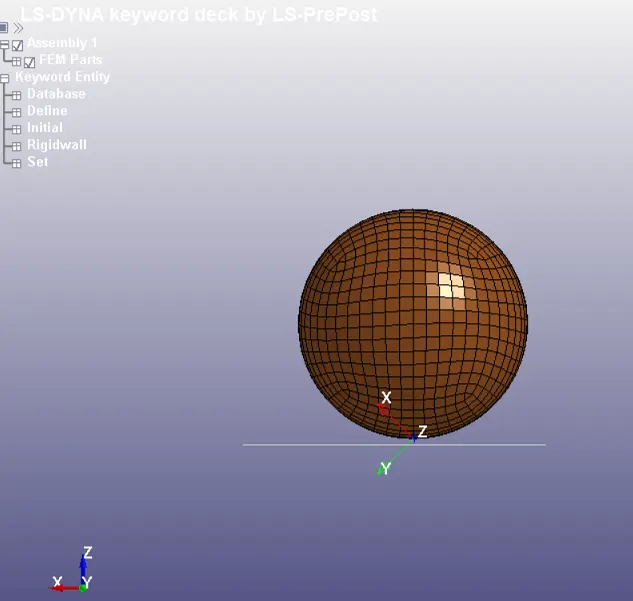
Fig 6: Coordinate system defined for initial velocity

• Case 2: A rigidwall was defined a few millimeters below the skin of the headform with a co-efficient of friction of 0.2. An initial velocity of 11.11mm/ms was provided to the entire headform model using Velocity_Generation and the predefined coordinate system 'initial_velocity'. Additionally, built-in within the headform file, were rigid bodies defined between the skull and accelerator block as well as the skull and backplate.

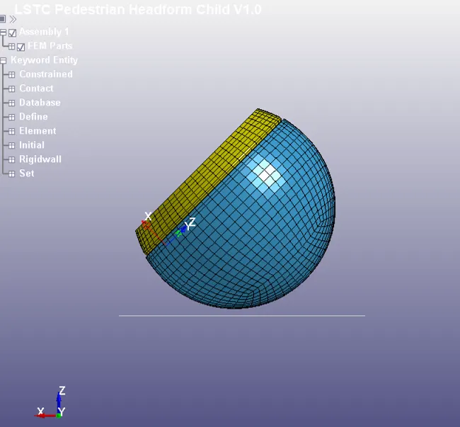
Fig 7: Coordinate system orientation for initial velocity

• Case 3: The initial velocity to the headform is provided the same way as in Case2. Since the rigidwall is replaced with the hood, the nodes along the edges of the hood were fixed along all dof using Boundary_SPC.

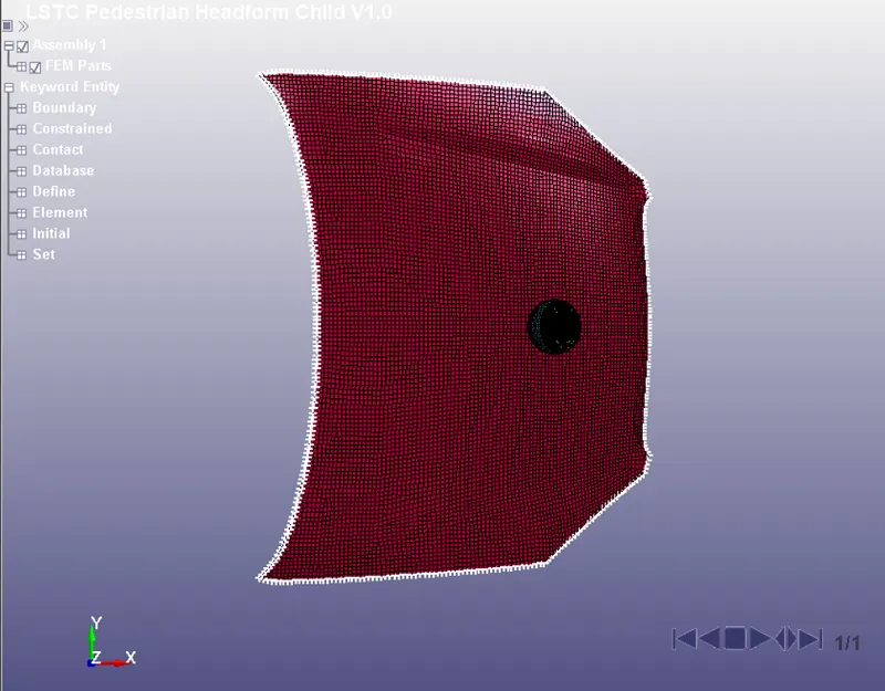
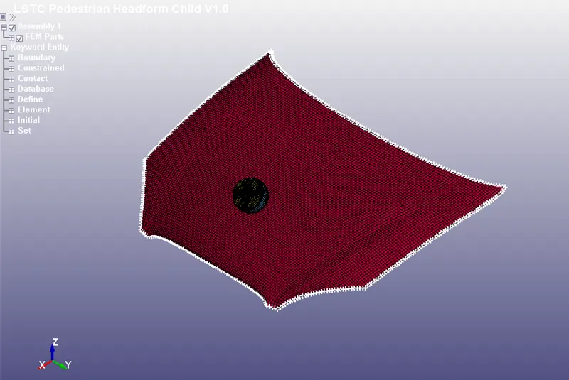
Fig 8: Fixed support SPC to the edge nodes of the hood

Contact Definition: An automatic surface-surface contact was already defined for the actual headform between the skin and the skull with a static and dynamic coefficient of friction of 0.8 each. An automatic single_surface contact was defined for the skin of the headform. For the simulation in case 3, an additional surface_surface contact was defined between the skin and the hood with a static and dynamic coefficient of friction of 0.2 and 0.15 respectively. The pre-defined Contact_control card settings were left to their default parameters.

Simulation Controls: The simulation was run for 60ms with a minimum timestep of 0.0011 for mass scaling (if necessary). Hourglass, Sliding contact, and rigidwall energies are requested for printing in the output file. Other pre-defined control cards are left to their default settings. The Binary plots and ASCII output files are requested at 1ms for case3 and 0.1ms for the other cases. The higher time for output requests for the third case was done to ensure faster computation of the problem. For the simulations using the actual headform model, node 25679 in the accelerometer block has been defined in Database_History_Node for nodout file printing.

Results and Discussion: All simulations terminate properly with appropriate energy balance ensured during the runs. For Case1, the stress and strain plots for element 15345 (at the bottom surface of the sphere) were plotted. The max effective stress noted was 0.48GPa and the mean integration point effective strain was 0.0021 at about 2ms i.e. right at the point of impact.

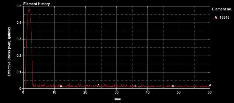
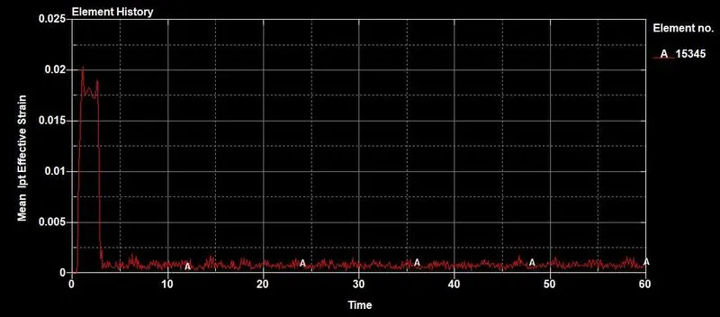
Fig 9: Stress plot for Case 1 Fig 10: Strain plot for Case 1

For Case2, the max effective stress (for element 2692) noted was about 0.012GPa and the max effective strain for the same element was 0.62. The stress and strain plots, in this case, were smoother than in case1 due to a better model of the headform with appropriate material cards.

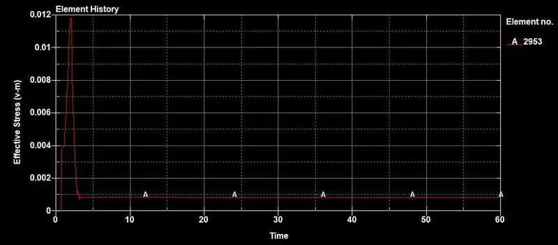
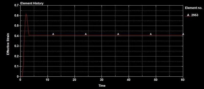
Fig 11: Stress plot for Case 2 Fig 12: Strain plot for Case 2

In Case 3, for element 2692, the max von-mises stresses recorded were 0.38GPa for all the impact points, although the variation of stress in the plot differed for each point. The max effective strain for the mean integration point of the element was recorded to be around 0.035, 0.052, and 0.05 for points 1, 2, and 3 respectively.

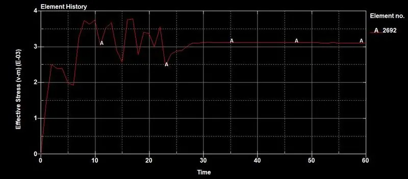
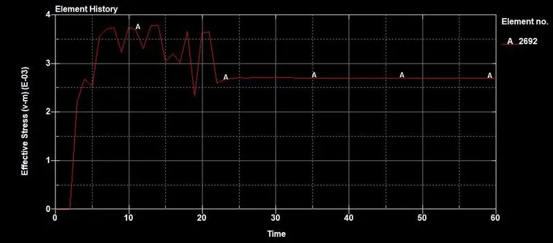
Fig 13: Stress plot for Case 3 point 1 Fig 14: Stress plot for Case 3 point 2

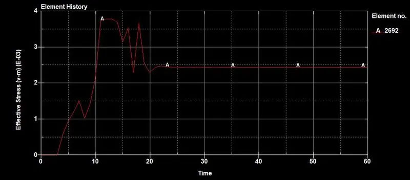
Fig 15: Stress plot for Case 3 point 3

The stress and strain rise in case 3 is over a longer period of time and it also levels out (at about 20ms) at a much higher value than in case2. In case two the peak stress and strains are recorded within the 5ms mark and they level out by the 10ms mark.

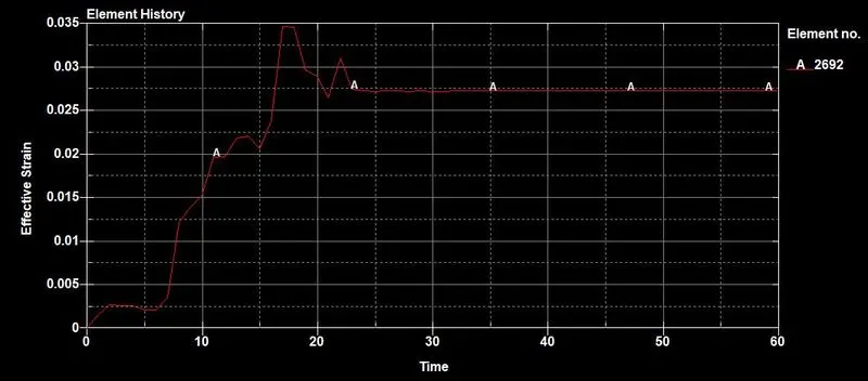
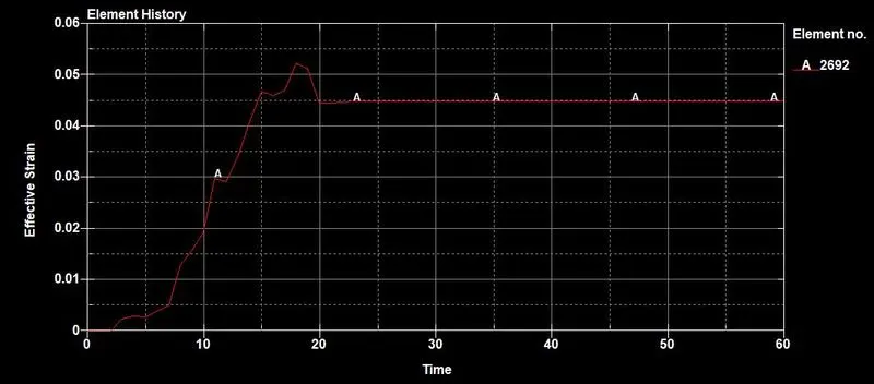
Fig 16: Strain plot for Case 3 point 1 Fig 17: Strain plot for Case 3 point 2

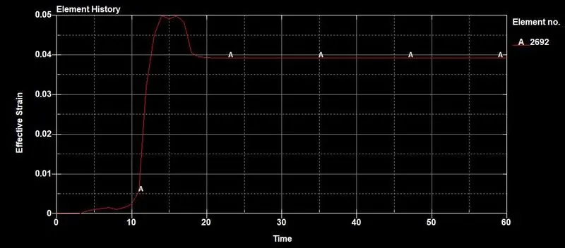
Fig 18: Strain plot for Case 3 point 3

The acceleration plot for case 1 (for node 68789) records a peak value of 450mm/ms2 between 1 and 2ms and after 3.5-4ms the acceleration fluctuates between 0 and 60-70mm/ms2 till the termination time. The corresponding HIC36 and HIC(d) values were 1.973e08 and 1.488e08 respectively. It is to be noted that these values are not reliable and redundant because of crude modelling and the fact that the HIC values were calculated for a time range that was less than 3ms.

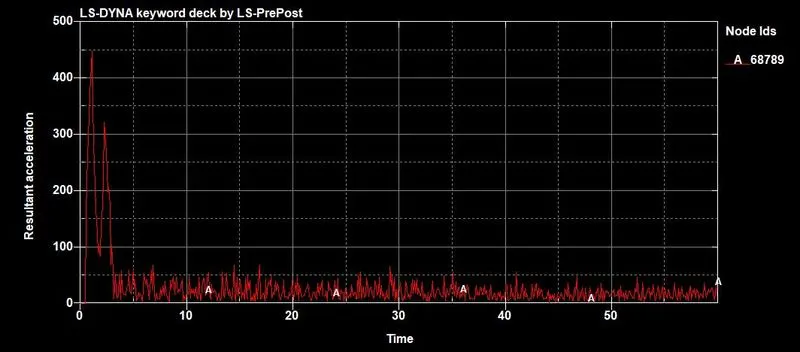
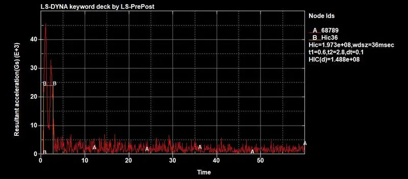
Fig 19: Acceleration plot for Case 1 Fig 20: HIC36 plot for Case 1

For Case 2, for the accelerometer node 25679, the peak value recorded was about 11.2mm/ms2 and the corresponding HIC36 and HIC(d) values were 2.541e04 and 1.934e04 respectively. These values are also not reliable since the deceleration takes place over a very short window and the HCI values have been calculated for a time range of 1ms only.

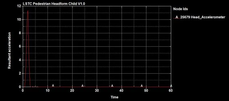
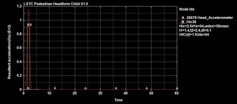
Fig 21: Acceleration plot for Case 2 Fig 22: HIC36 plot for Case 2

For Case 3, for the node 25679, the peak accelerations recorded were 1.35mm/ms2, 1.12mm/ms2 and 1.6mm/ms2 for points 1, 2 and 3 respectively. The acceleration and deceleration also take place over a longer time period than in the previous cases - over approximately 20-25ms range.

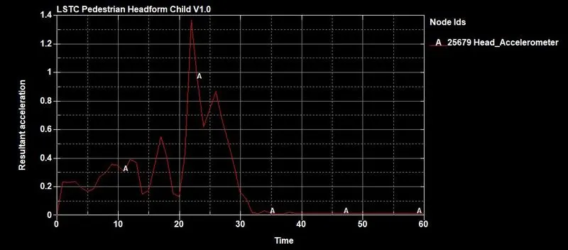
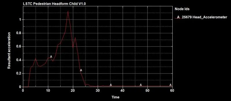
Fig 23: Acceleration plot for Case 3 point 1 Fig 24: Acceleration plot for Case 3 point 2

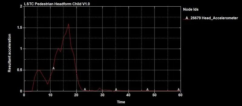
Fig 25: Acceleration plot for Case 3 point 3

The HIC36 and HIC(d) values computed were 441 and 499.2 for point1 (t1-t2 = 7ms), 451.5 and 507.1 for point 2 (t1-t2 = 11ms), and 1062 and 967.5 for point 3 (t1-t2=9ms) respectively.

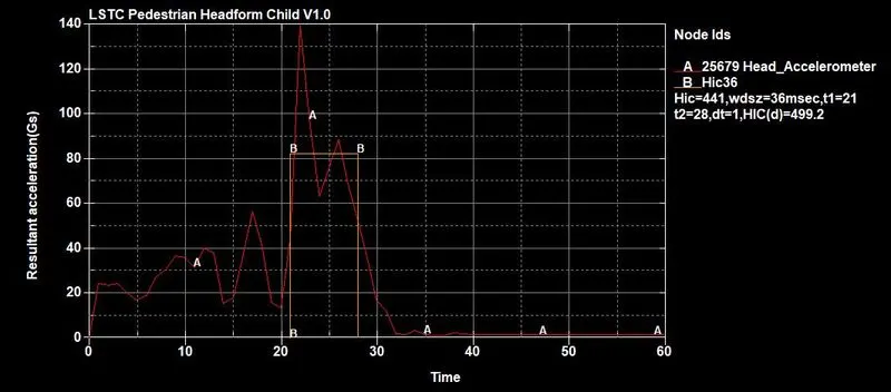
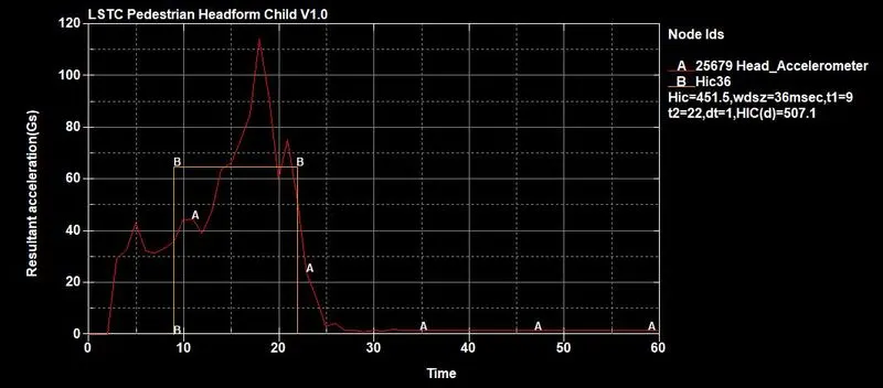
Fig 26: HIC36 plot for Case 3 point 1 Fig 27: HIC36 plot for Case 3 point 2

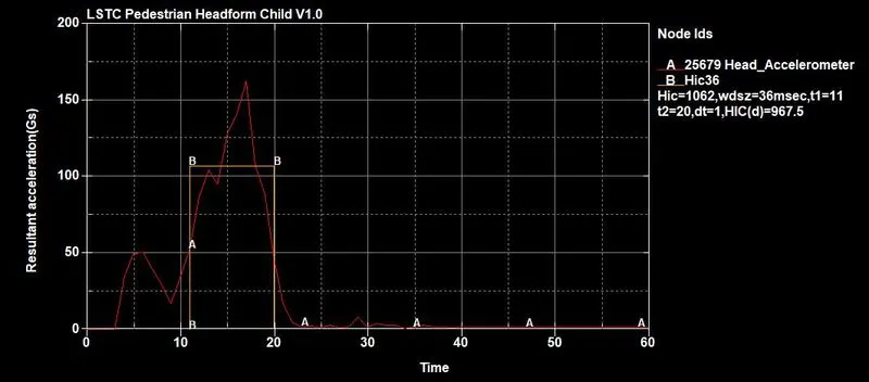
Fig 28: HIC36 plot for Case 3 point 3

Conclusion: As can be observed from the HIC and acceleration plots above, the most reliable and realistic values of HIC were obtained from Case3. This is quite obviously because of the more accurate modelling with an actual headform and a hood (instead of a rigidwall). From Fig 28 it can be seen that the HIC36 value for point 3 crosses 1000 mark and the HIC (d) value is quite close to 1000 indicating a very high probability of level 6 or serious injury if the pedestrian head impacts that point. For the other two impact points, the HIC values are within a reasonable 500-510 range. Further studies can be conducted to compute the extent of intrusion of the hood sheet metal panel into the engine compartment and check for sufficient clearance with the engine components.