Week-7 Head Impact
Assignment 7
This assignment is dedicated to the simulation of a head impact on a car hood. Three different scenarios will be considered.
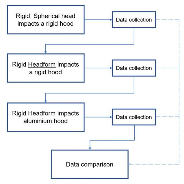
The workflow of this assignment will be the following:
1. Model setup
A main file was created to mate all the components involved in the crash. The main file is MAIN.k.
Inside this file, the *INCLUDE keyword was activated twice to join the information about the meshes of the hood and the head in the same file. The next image shows both parts in the MAIN.k file:
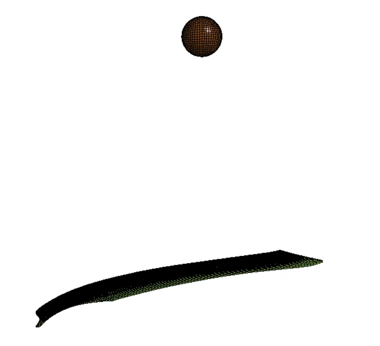
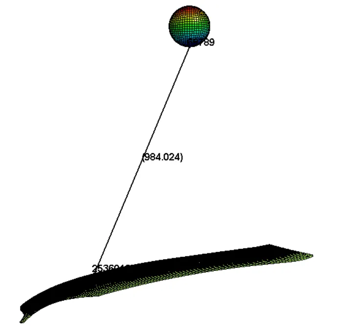
It can clearly be seen that the head is too far away to the hood to simulate a realistic crash situation. Therefore, inside the Simple_Head_Model.k file,by using the Element Tools>Transform option, the head was put in a more realistic position for this situation (see figure to the right).
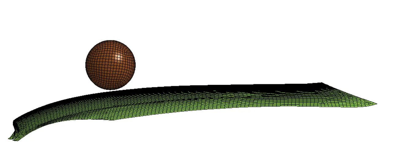
For scenarios 2 and 3, the Headform was placed, roughly 40 mm away from the hood, as shown below.
2. Material definition
The material for all the simulations to be performed are the following:
- Hood and Head: Aluminium (The material was defined right away but this configuration will only be used in the third scenario. In the first two scenarios, a rigid body will be attached to the hood to force it to have a rigid material behaviour).
- Young's Modulus:
`E = 70 GPa = 70\times10^9 \frac{N}{m^2} = 70\times10^9 \frac{Kg \times m/s^2}{(1000 mm)^2} = 70\times10^9 \frac{0.001 \t\o\n \times 1000 mm/s^2}{(1000 mm)^2} = 70 000 \frac{\t\o\n {mm}/s^2}{(mm]^2}`
- Density:
`\rho = 2700 {Kg}/m^3 = 2.7 \frac{\t\o\n}{(1000 mm)^3} = 2.7 \times 10^{-9} frac{\t\o\n}{mm^3}`
- Poisson Coefficient:
`\nu = 0.33`
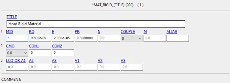
The image below show the definition of the rigid material for the head and for the hood:
To define the elasto-plastic material for the aluminum hood, a csv. file containing measurements from a tensile test of a 6061-T651 aluminium alloy was obtained (https://data.mendeley.com/datasets/rd6jm9tyb6/2) and the data was used as an imput to a simple MatLab program to calculate the yield stress.
The following pictures shows the obtained data:
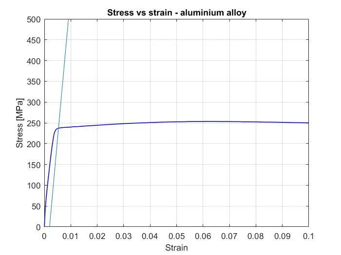
The yield stress at 0.2% strain was calculated to be 244 MPa, and that value was used in the field SIGY.
This data was used to export the values (stress,strain) to a .csv file to be imported to LS Dyna as a curve:
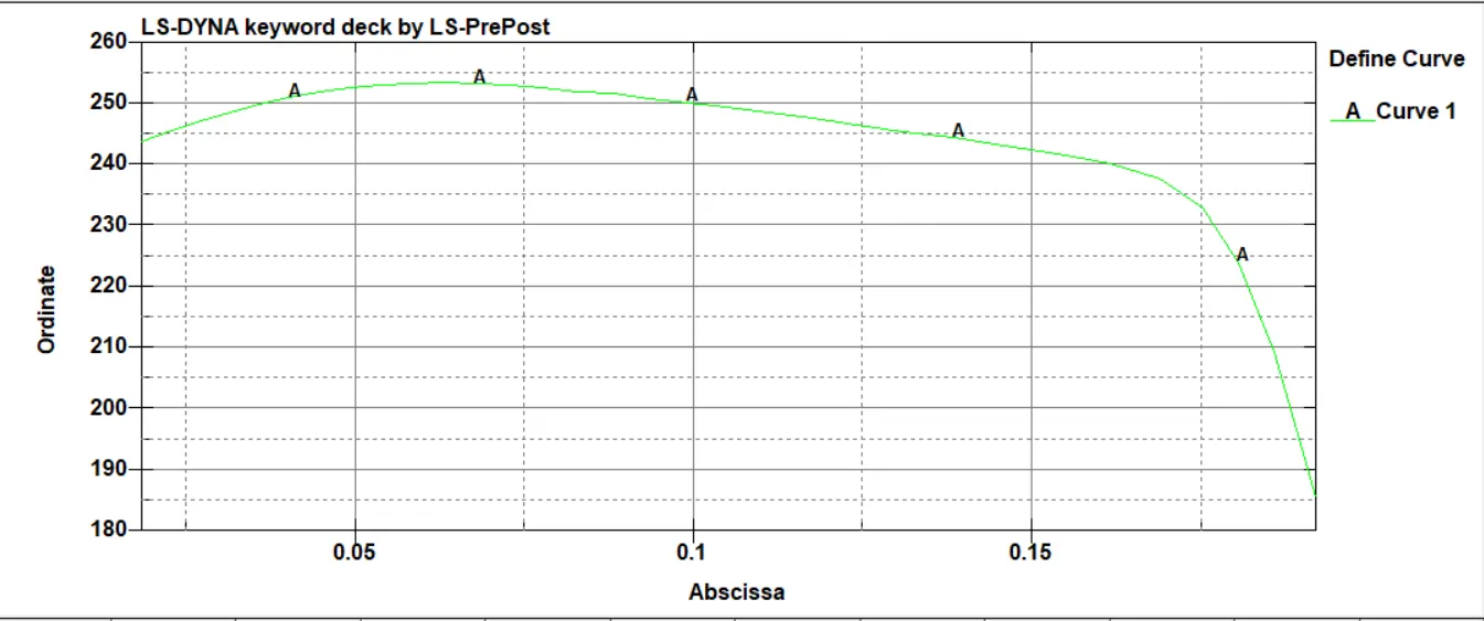
Only the post-yield section of the curve is represented, because all the parameters of the linear section of the curve were given to the program.
An error arose from the fact that the slope between, at least, two points of the curve was negative. To correct this issue, the negative slope section of the slope was deleted, resulting in the following curve:
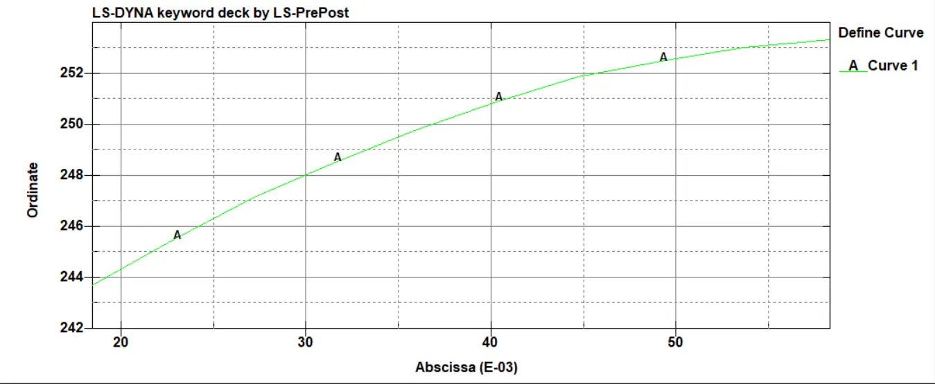
This curve was then associated to the *MAT_PIECEWISE_LINEAR_PLASTICITY to complete the definition of this material keyword.
The data of this curve was used for scenario 1. For scenraios 2 and 3, the values of the stress were changed to GPa.
3. Section definition
To define both sections, a thickness of 3 mm was associated to the simple head and hood. Besides that, the element formulation ID was set to 2 (Belytschko-Tsay).
The sections defined for the Headform model remained the same.
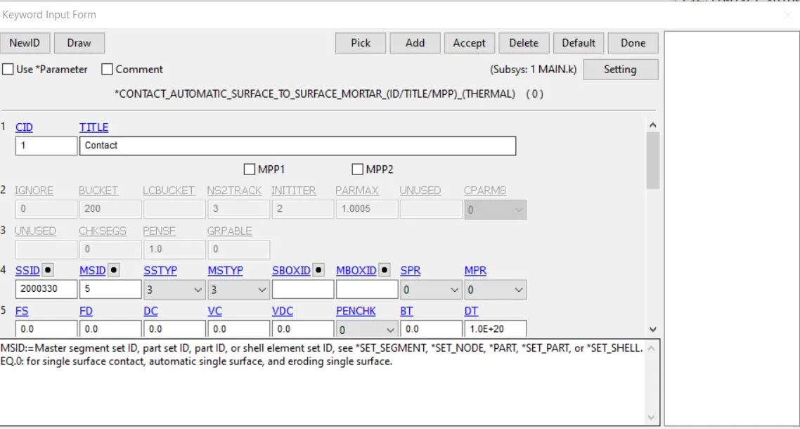
4. Contact definition
An automatic surface to surface type of contact. This contact was chosen for reasons of simplicity.
5. Initial velocity
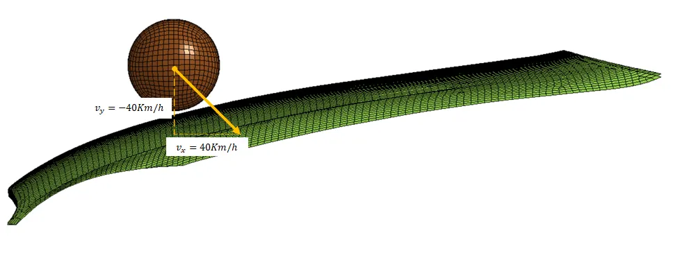
An initial velocity vector is imposed to the head of the pedestrian. The vector of the initial velocity must comply with two requirements:
- Its inclination must be between 35º and 75º with the horizontal (or x) direction
- Its horizontal magnitude must be between 20 and 40 Km/h
This vector was defined in a way that the horizontal component of the velocity is 40 Km/h (= 11111 mm/s = 11.11 mm/ms). Its inclination with the horizontal direction was set at 45º, meaning that the vertical component of the velocity also has a value of 40 Km/h.
5. Rigid body (for scenario 1)
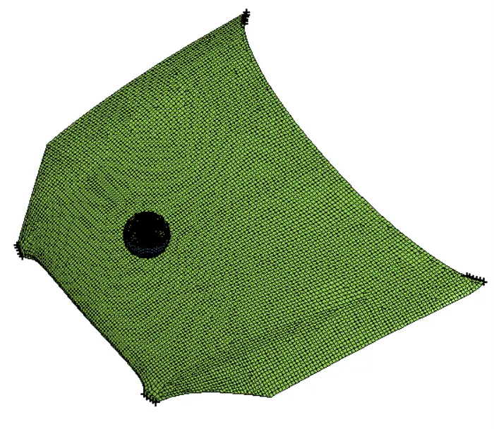
For the first case approached in this assignment, it is necessary to consider the hood as a rigid wall. This is done by creating a Centre-Node Rigid Body that connects all the nodes of the hood to a central one and prevents them from moving relatively to each other. The next figure shows the rigid body that was created.
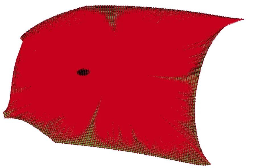
The centre node of the rogod body was constrained.
For scenario 3, only the hood supports were contrained:
6. Controls
The CONTROL_TERMINATION keyword was activated. In this keyword, the total simulation time must be defined, to calculate the total simulation time, first, we need to understand the expected time for the collision, and then slightly increase that time.
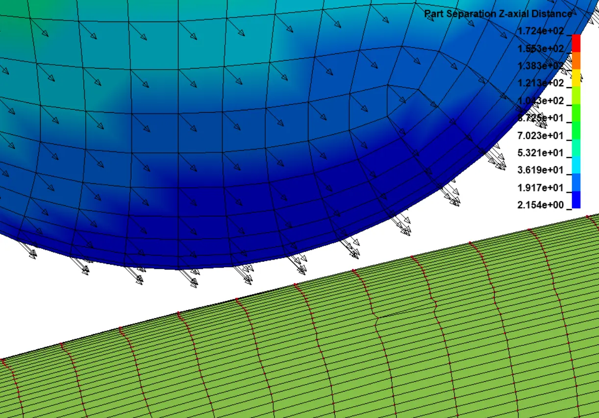
As shown in the following figure, the initial distance between the head and the hood is 2.154 mm. The collision time can be calculated as follows:
`v = \sqrt{v_x^2+v_y^2}=\sqrt{11111^2+11111^2} = 15713 {mm}/s`
`t_{collision}=\frac{\Deltad}{v} = \frac{2.154}{15713}=0.000137 s`
A reasonable time to the simulation is 0.1 s for scenario 1.
Scenarios 2 and 3 were analysed with a simulation time of 50 ms.
7. Outputs
It is important to collect the strain and stress plots from all the simulations performed in this assignment. Therefore, the DATABASE_EXTENT_BINARY and DATABASE_BINARY_D3PLOT keywords were activated.
8. Results
8.1. Scenario 1 - Simple Head model hits rigid hood
As expected, the impact happens right at the beginning of the simulation because the head was placed very close to he hood.
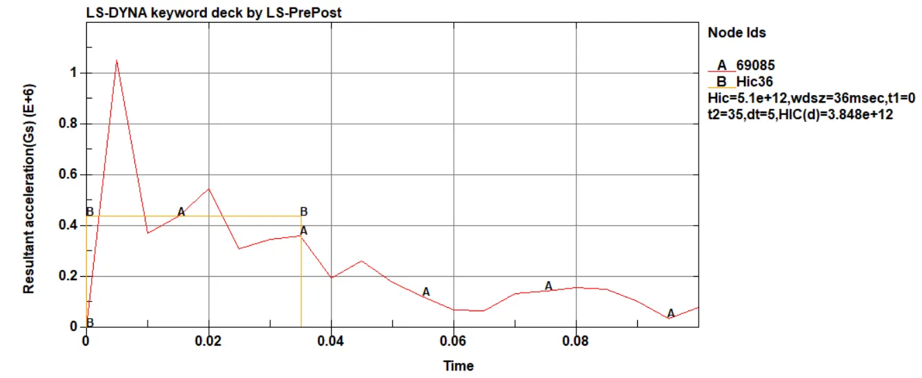
the HIC can also be calculated manually, as follows:
`HIC = [\frac{1}{t_2-t_1}\int_{t_1}^{t_2}\overline{a}(t)dt]^2.5(t_2-t_1) = [\frac{1}{0.036}\int_{0}^{0.036}1.05\times10^{6}dt]^2.5\times0.036 = 4.067\times10^13`
8.2. Scenario 2 - Headform hits rigid hood
The impact peak acceleration lasted for less than 3 ms. Meaning that the program was unable to capture valid data to calculate the HIC.
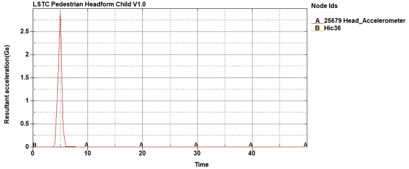
Nevertheless, the HIC can be calculated manually, using the maximum acceleration value: `a = 29.1 \frac{mm}{ms^2}`:
`HIC = [\frac{1}{t_2-t_1}\int_{t_1}^{t_2}\overline{a}(t)dt]^2.5(t_2-t_1) = [\frac{1}{0.036}\int_{t_1}^{t_2}29.1/0.0098dt]^2.5\times0.036 = 1.73 times 10^7`
Right away, it can be seen that the order of magnitude of the latter value of the HIC is much smaller compared to the first one. But this is only due to the fact that different unit systems were used.
8.3. Scenario 3 - Headform hits aluminium hood
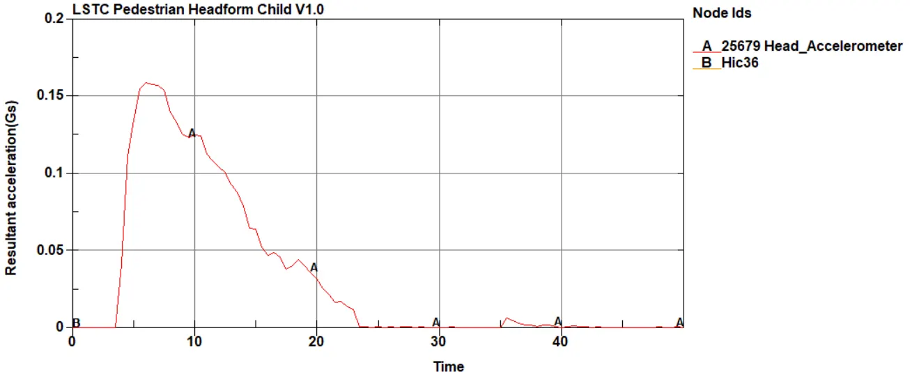
Despite of the missing HIC in this plot, the approximate value can also be calculated by hand:
`HIC = [\frac{1}{t_2-t_1}\int_{t_1}^{t_2}\overline{a}(t)dt]^2.5(t_2-t_1) = [\frac{1}{0.036}\int_{t_1}^{t_2}5.06\times10^3/0.0098dt]^2.5\times0.036 = 6.9\times10^{-12}`
9. Conclusions
- Sometimes, the HIC was not obtained. I belive that the main reason for this is the fact that the peak acceleration last less than 3 ms. But then, I realized that there could be something wrong with the program output request. After searching for what could possibly be wrong, the reason for the HIC not to be shown in the plots remains unanswered.
- When the hood was modelled as an aluminium part instead of a rigid one, the time-span for the acceleration of the head increased significantly, meaning that the stiffer the hood, the higher the peak acceleration value.