Week 7 - Auto ignition using Cantera

Auto ignition using Cantera

Objectives:

PART I

Program a reactor network code to simulate the Auto Ignition Time for Methane under the following conditions (simulation time = 10 secs)

• Plot the variation of the Auto Ignition time of Methane with a constant temperature of 1250K and pressure varying from 1 to 5 atm.
• Plot the variation of the Auto Ignition time of Methane with a constant pressure of 5 atm and temperature varying from 950K to 1450K.

PART II

Observe and print the rate of change of molar concentrations of the given elements "H2O, O2, OH" with respect to the time (simulation time = 10 secs)

Analyze the behavior of the graph for 2 cases,

• When Temperature is 1000K, and the pressure is 5 bar
• When Temperature is 500K, and the pressure is 5 bar

Auto Ignition Temperature & Ignition delay:

It is the lowest temperature at which ignition takes place. Ignition delay is the time required for ignition to take place. It depends on temperature, pressure & mixture composition.

Ignition delay has to be optimum. If it happens at a larger time scale, then some of the above-mentioned parameters are not favorable, or the fuel-air mixture is either lean or rich.

In certain cases, Ignition delay happens at higher temperatures, but at low-temperature, combustion occurs. This is known as the Negative temperature coefficient.

So theoretically, Auto Ignition time is the time when the temperature of the reactor is at Initial Temperature plus 400K.

Variation of Auto Ignition time of Methane with a constant temperature of 1250K and pressure varying from 1 to 5 atm:

"Variation of Auto Ignition time of Methane with a constant temperature"

import sys
import numpy as np
import cantera as ct
import matplotlib.pyplot as plt

gas = ct.Solution('gri30.xml')
T=1250
P = [1,2,3,4,5]
ignition_delay=[]

for i in range(len(P)):
    gas.TPX = T,P[i]*101325,{'CH4':1,'O2':2,'N2':7.52}
    r=ct.IdealGasReactor(gas)
    sim = ct.ReactorNet([r])
    time=0
    "gives an object that describes the states of the reactor objects"
    states = ct.SolutionArray(gas,extra=['time_in_ms','t'])

    for n in range(10*1000):
        "this is not a timestep, cantera computes/integrates till this time state, time step is chosen by cantera itself"
        time += 1e-3
        sim.advance(time)
        states.append(r.thermo.state, time_in_ms = time*1e3, t=time)

    for j in range(len(states.T)):
        if states[j].T >= 1250+400: #Auto Ignition time is the time when the temperature of the reactor is Initial Temperature plus 400K.
            ignition_delay.append(states.time_in_ms[j])
            break


plt.plot(P,ignition_delay,marker='D')
plt.xlabel('Pressure in bar')
plt.ylabel('ignition delay in ms')
plt.show()

Output:

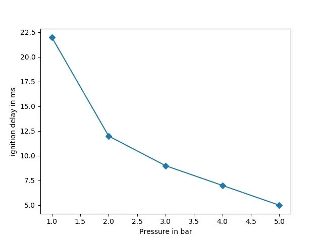
Inference: Ignition delay decreases when pressure increases.

Variation of Auto Ignition time of Methane with a varying temperature and constant pressure:

"Variation of Auto Ignition time of Methane with a constant pressure"

import sys
import numpy as np
import cantera as ct
import matplotlib.pyplot as plt

gas = ct.Solution('gri30.xml')
T=np.linspace(950,1450)
P = ct.one_atm*5
ignition_delay=[]

for i in range(len(T)):
    gas.TPX = T[i],P,{'CH4':1,'O2':2,'N2':7.52}
    r=ct.IdealGasReactor(gas)
    sim = ct.ReactorNet([r])
    time=0
    "gives an object that describes the states of the reactor objects"
    states = ct.SolutionArray(gas,extra=['time_in_ms','t'])

    for n in range(10*1000):
        "this is not a timestep, cantera computes/integrates till this time state, time step is chosen by cantera itself"
        time += 1e-3
        sim.advance(time)
        states.append(r.thermo.state, time_in_ms = time*1e3, t=time)

    for j in range(len(states.T)):
        if states[j].T >= 1250+400:
            ignition_delay.append(states.time_in_ms[j])
            break


plt.plot(T,ignition_delay,marker='D')
plt.xlabel('Temperature in K')
plt.ylabel('ignition delay in ms')
plt.show()

Output:

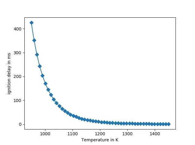
Inference: Ignition delay decreases as temperature increases.

Rate of change of molar concentrations of the given elements "H2O, O2, OH" with respect to the time:

"Rate of change of molar concentrations of the given elements H2O, O2, OH with respect to the time"

import sys
import numpy as np
import cantera as ct
import matplotlib.pyplot as plt

gas = ct.Solution('gri30.xml')
T=[500,1000]
P=5*101325

for i in range(len(T)):
    print(i)
    gas.TPX = T[i],P, {'CH4':1,'O2':2,'N2':7.52}
    r=ct.IdealGasReactor(gas)
    sim = ct.ReactorNet([r])
    time=0

    "gives an object that describes the states of the reactor objects"
    states500 = ct.SolutionArray(gas,extra=['time_in_ms','t'])
    states1000 = ct.SolutionArray(gas,extra=['time_in_ms','t'])


    for n in range(10*1000):
        "this is not a timestep, cantera computes/integrates till this time state, time step is chosen by cantera itself"
        time += 1e-3
        sim.advance(time)
        states500.append(r.thermo.state, time_in_ms = time*1e3, t=time)
        states1000.append(r.thermo.state, time_in_ms = time*1e3, t=time)


    if i==0:

        plt.subplot(3,1,1)
        plt.plot(states500.t,states500.X[:,gas.species_index('H2O')],color = 'blue')
        plt.title("At T=500K")
        plt.ylabel('Concentration of H2O')

        plt.subplot(3,1,2)
        plt.plot(states500.t,states500.X[:,gas.species_index('O2')],color = 'green')
        plt.ylabel('Concentration of O2')

        plt.subplot(3,1,3)
        plt.plot(states500.t,states500.X[:,gas.species_index('OH')],color = 'red')
        plt.xlabel('Time (s)')
        plt.ylabel('Concentration of OH')
        plt.show()

    if i==1:

        plt.subplot(3,1,1)
        plt.plot(states1000.t,states1000.X[:,gas.species_index('H2O')],color = 'blue')
        plt.title("At T=1000 K")
        plt.ylabel('Concentration of H2O')

        plt.subplot(3,1,2)
        plt.plot(states1000.t,states1000.X[:,gas.species_index('O2')],color = 'green')
        plt.ylabel('Concentration of O2')

        plt.subplot(3,1,3)
        plt.plot(states1000.t,states1000.X[:,gas.species_index('OH')],color = 'red')
        plt.xlabel('Time (s)')
        plt.ylabel('Concentration of OH')
        plt.show()

Output:

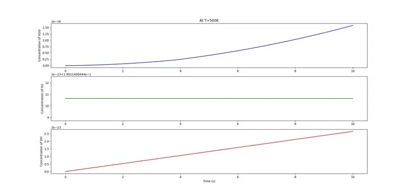
Inference at T=500K: The concentration of H2O is increasing exponentially, and the concentration of OH is increasing in a linear pattern, whereas the concentration of O2 is almost constant at around 10.8 moles.

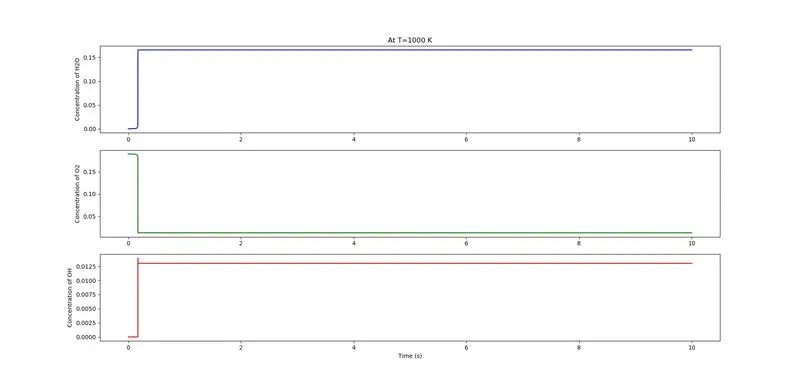
Inference at T=1000K: The concentration of H2O is increasing abruptly to 0.15 moles and remains constant, and the concentration of OH possesses the same pattern of H2O at 0.0125 moles, whereas the concentration of O2 is decreased to near zero.

Observations:

• Studies were performed to explore the behavior of ignition delay with respect to temperature and pressure. It is evident from the plots that either increase in temperature or pressure reduces the ignition delay for methane. However, this may not be true for other species.
• At lower temperatures, concentrations of H2O and OH are not converged and remain at an increasing trend, whereas at a much higher temperature of around 1000K, the methane undergoes combustion, and the concentration of H20 and OH stays constant after a rapid surge initially.
• The concentration of O2 stays constant at lower temperatures, but at higher temperatures, it reduces in concentration.