Week 7 - Auto ignition using Cantera

OBJECTIVES:- To solve the challenge of Auto-ignition by using Python with Cantera.

PROBLEM STATEMENTS:-

PART-A

Use the same reactor network code as shown in the video to simulate the auto-ignition Time for methane under the following conditions, (Simulation time = 10 Secs).

Plot the variation of auto-ignition time of methane with a constant temperature of 1250k and pressure varying from 1 to 5 atm.

Plot the variation of auto-ignition time of methane with a constant pressure of 5 atm and temperature varying from 950k to 1450k.

NOTE:- auto-ignition time is the time when the temperature of the reactor is Initial temperature plus 400K.

“Time of auto-ignition delay = Time of initial temperature + 400k”.

PART-B

Further observe and print the rate of change of molar concentration of the given elements “H2O, O2, OH” with respect to the time, (simulation time = 10 secs).

Explain the behavior of the graph for 2 cases,

When the temperature is 1000k and pressure 5 bar

When the temperature is 500k and pressure is 5 bar

INTRODUCTIONS & THEORY:-

The autoignition temperature or kindling point of a substance is the lowest temperature in which it spontaneously ignites in a normal atmosphere without an external source of ignition, such as flame or spark. This temperature is required to supply the activation energy needed for combustion.

Following are the general questions regarding auto-ignition are as follows-

The applications of controlled auto-ignition Gasoline Engines –The challenges and solutions:-

Controlled auto-ignition (CAI) combustion, also known as Homogeneous Charge Compression Ignition (HCCI), has the potential to simultaneously reduce the fuel consumption and nitrogen oxide emissions of gasoline engines. However, a narrow operating region in loads and speeds is one of the challenges for the commercial application of CAI combustion. The effect of intake charge boosting, charge stratification, and spark-assisted ignition on the operating range in CAI mode was reviewed. A stratified flame ignited (SFI) hybrid combustion is one form to achieve CAI combustion under the conditions of a highly diluted mixture caused by the flame in the stratified mixture with the help of a spark plug. CAI combustion in a two-stroke gasoline engine can be used to enhance the torque of a four-stroke gasoline engine with the same displacement at the same indicated mean effective pressure. Poppet valved two-stroke gasoline engines with normal valve lift and variable valve timing device, and uniflow two-stroke engines with gas exchange process completed by intake ports on the bottom of the cylinder wall and overhead exhaust poppet valves are promising to achieve CAI combustion in a wide operating range. Hence, CAI combustion in a two-stroke gasoline engine is a feasible solution for its commercial application to vehicles.

STEPWISE PROCEDURES OF CODE:-

There have different cases for writing code but, I write here common steps to involved in writing code.

1. First off all imported all different modules used in the code like sys, numpy, Cantera, and matplotlib.
2. Then define a gas solution
3. Then define temperature & pressure.
4. Use for loop and define temperature, pressure, and molar concentrations.
5. Use the reactor as IdealGasReactor and simulation reactor as ReactorNet.
6. The time range is between 0.0 to 10.0 seconds i.e. 10000ms, which is the time step size.
7. Use the states as SolutionArray
8. The solution to be calculated at every 1e-3 sec
9. Integrate system to the time given
10. Then creating if loop for finding the ignition delay
11. If the new temperature is greater than or equal to 400 + old temperature, then and then print ignition delay.
12. Plots two graphs are (states.t, states.T) and (Temp, Ignition delay).

PART- A

Code at constant Pressure:-

import sys
import numpy as np 
import cantera as ct 
import matplotlib.pyplot as plt 

gas = ct.Solution("gri30.xml")
T_i = 950
T_e = 1450
Temp = np.linspace(T_i,T_e,11)
Ignition_delay = []
P = 5*101325  # Pressure should be defined in Pascal. Cantera uses SI unit
for T in Temp:
	
	gas.TPX = T,P,{'CH4':1,'O2':2, 'N2':7.52}
	r = ct.IdealGasReactor(gas) # Ideal gas reactor is the class and r is instance of it
	sim = ct.ReactorNet([r]) # Creating the simulation object
	time = 0.0
	T_old = T
	states = ct.SolutionArray(gas,extra=['time_in_ms','t']) 
	i=1
	for i in range(1000): 
		time+=1e-3 
		sim.advance(time) #Integrate system to the time given
		states.append(r.thermo.state,time_in_ms = time*1e3, t=time)
		T_new = states.T
		T_new = T_new[i-1]
		
		#creating if loop for finding the ignition delay
		#(Time)ignition delay = (Time)initial temp + 400K
		if (T_new>=400+T_old):
			Ignition_delay.append(time)
			
			T_old = states.T
			T_old = T_old[i-1]

			plt.figure(1)
			plt.plot(states.t,states.T)


plt.legend(['Temp = ' + str(T) + '[k]' for T in Temp])
plt.xlabel('Time')
plt.ylabel('Temperature')
print('Ignition_delay = ',Ignition_delay)
plt.savefig("Temperature Vs Time")

plt.figure(2)
plt.plot(Temp,Ignition_delay,'-*')
plt.xlabel('Temperature [K]')
plt.ylabel('Ignition_delay [ms]')
plt.savefig("Ignition delay vs temperature")
plt.show()

Code at constant Temperature:-

import sys
import numpy as np 
import cantera as ct 
import matplotlib.pyplot as plt 

gas = ct.Solution("gri30.xml")
P_i = 1*101325
P_e = 5*101325
Press = np.linspace(P_i,P_e,11)
Ignition_delay = []
T = 1250  # Pressure should be defined in Pascal. Cantera uses SI unit
for P in Press:
	
	gas.TPX = T,P,{'CH4':1,'O2':2, 'N2':7.52}
	r = ct.IdealGasReactor(gas) # Ideal gas reactor is the class and r is instance of it
	sim = ct.ReactorNet([r]) # Creating the simulation object
	time = 0.0
	T_old = T
	states = ct.SolutionArray(gas,extra=['time_in_ms','t']) # As gases are in different temperature and pressure at instance
	i=1
	for i in range(1000): #Time step size = 10s
		time+=1e-3 #Solution to be calculated at every 1e-3s
		sim.advance(time) #Integrate system to the time given
		states.append(r.thermo.state,time_in_ms = time*1e3, t=time)
		T_new = states.T
		T_new = T_new[i-1]
		
		#creating if loop for finding the ignition delay
		if (T_new>=400+T_old):
			Ignition_delay.append(time)
			
			T_old = states.T
			T_old = T_old[i-1]


			plt.figure(1)
			plt.plot(states.t,states.T)


# plt.legend(['Temp = ' + str(T) + '[k]' for T in Temp])
plt.xlabel('Time')
plt.ylabel('Temperature')
print('Ignition_delay = ',Ignition_delay)
plt.figure(2)
plt.plot(Press/1000, Ignition_delay,'-*')
plt.xlabel('Pressure x 10^3 [Pa]')
plt.ylabel('Ignition_delay [ms]')
plt.show()
plt.show()

PART- B

Here molar concentrations are “H2O, O2 & OH” with respect to time.

Code at Temp = 1000k & 5 bar :-

import sys
import numpy as np 
import cantera as ct 
import matplotlib.pyplot as plt 

Temp = [1000]
for T in Temp:
	gas = ct.Solution("gri30.xml")
	P = 5*101325
	gas.TPX = T,P,{'CH4':1,'O2':2, 'N2':7.52}
r = ct.IdealGasReactor(gas) # Ideal gas reactor is the class and r is instance of it
sim = ct.ReactorNet([r]) # Creating the simulation object
time = 0.0
T_old = T
states = ct.SolutionArray(gas,extra=['time_in_ms','t']) # As gases are in different temperature and pressure at instance
i=1
for i in range(10000): #Time step size = 10s
	time+=1e-3 #Solution to be calculated at every 1e-3s
	sim.advance(time) #Integrate system to the time given
	states.append(r.thermo.state,time_in_ms = time*1e3, t=time)

#Plot rate of H2O Mole fraction
plt.subplot(1,3,1)
plt.plot(states.t, states.X[:, gas.species_index("H2O")])
plt.xlabel("Simulation time")
plt.legend(["H2O-Mole fraction"])
plt.title("Rate of concentration of H2O")

#Plot Rate of O2 Molar fraction
plt.subplot(1,3,2)
plt.plot(states.t, states.X[:,gas.species_index("O2")])
plt.xlabel("Simulation time")
plt.legend(["O2-Mole fraction"])
plt.title("Rate of concentration of O2")

#Plot rate of OH Molar fraction
plt.subplot(1,3,3)
plt.plot(states.t, states.X[:, gas.species_index("OH")])
plt.xlabel("Simulation time")
plt.legend(["OH-Molefraction"])
plt.title("Rate of concentration of OH")
plt.suptitle("Rate of change of concentration of H2O, O2 & N2 at" + str(T) + "[Kelvin")
plt.savefig("Plot for 1000k")
plt.show()

Code at Temp = 500k & 5 bar :-

import sys
import numpy as np 
import cantera as ct 
import matplotlib.pyplot as plt 

Temp = [500]
for T in Temp:
	gas = ct.Solution("gri30.xml")
	P = 5*101325
	gas.TPX = T,P,{'CH4':1,'O2':2, 'N2':7.52}
r = ct.IdealGasReactor(gas) # Ideal gas reactor is the class and r is instance of it
sim = ct.ReactorNet([r]) # Creating the simulation object
time = 0.0
T_old = T
states = ct.SolutionArray(gas,extra=['time_in_ms','t']) # As gases are in different temperature and pressure at instance
i=1
for i in range(10000): #Time step size = 10s
	time+=1e-3 #Solution to be calculated at every 1e-3s
	sim.advance(time) #Integrate system to the time given
	states.append(r.thermo.state,time_in_ms = time*1e3, t=time)
	
#Plot rate of H2O Mole fraction
plt.subplot(1,3,1)
plt.plot(states.t, states.X[:, gas.species_index("H2O")])
plt.xlabel("Simulation time")
plt.legend(["H2O-Mole fraction"])
plt.title("Rate of concentration of H2O")

#Plot Rate of O2 Molar fraction
plt.subplot(1,3,2)
plt.plot(states.t, states.X[:,gas.species_index("O2")])
plt.xlabel("Simulation time")
plt.legend(["O2-Mole fraction"])
plt.title("Rate of concentration of O2")

#Plot rate of OH Molar fraction
plt.subplot(1,3,3)
plt.plot(states.t, states.X[:, gas.species_index("OH")])
plt.xlabel("Simulation time")
plt.legend(["OH-Molefraction"])
plt.title("Rate of concentration of OH")
plt.suptitle("Rate of change of concentration of H2O, O2 & N2 at" + str(T) + "[Kelvin")
plt.savefig("Plot for 500k")
plt.show()

RESULTS:-

PART-A

Below we can see the plot of methane under the variation of temperature and constant pressure, the below plots gave the variation of temperature given time.

Observing the plot the temperature increases, as well as ignition delay decreases. At initial temperature needs more time to auto-ignite. That we can see below the graph, if the temperature is low, the ignition delay is high, and the initial temperature is high, the ignition delay is low. As compared to the pressure the ignition delay is faster because of the temperature high. It may help with the auto-ignition.

CASE-1:- At constant pressure-

1. Ignition delay vs temperature:-

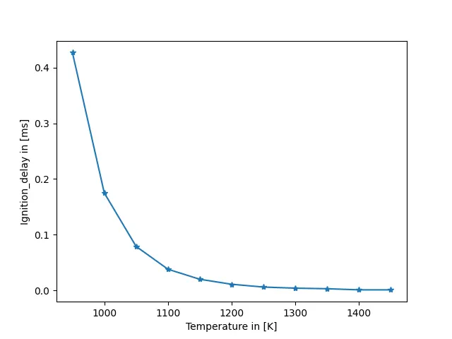
The above figure predicts that, ignition delay vs temperature. The graph change is parabolic. As temperature increases, ignition delay decreases and vice versa. At the start, ignition delay decreases very fastly and later on tends to constant. Due to a sudden increase in temperature, the ignition delay occurs because of an improper mixture of air fuel or incomplete combustion of the air-fuel mixture.

2. Temperature vs time:-

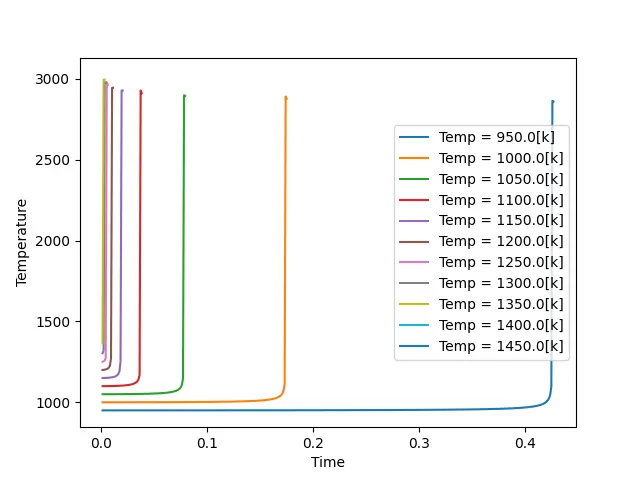
From the above figure, we can see that, temperature variation at different times. We can see that temperature change is constant every time. Here, we analyze that, ignition delay at each time is constant. From left to right, ignition delay increases but, the temperature remains constant.

At the start, temperature delay is increased as time decreases.

CASE-2:- At constant temperature-

1. Ignition delay vs pressure:-

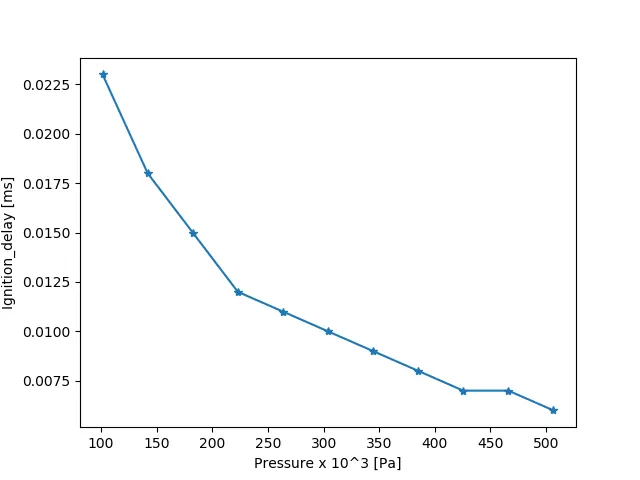
The above figure depicts that, the graph Ignition delay vs pressure. As ignition delay decreases, pressure increases and vice versa. At start ignition delay decreases very fast but, as pressure increases ignition delay decreases gradually. This change is called logarithmic change.

As we know that, the temperature is inversely proportional to pressure. At the start of ignition delay, the temperature is maximum, and that why pressure is minimum. Ignition delay decreases slowly as pressure increases.

2. Temperature vs time:-

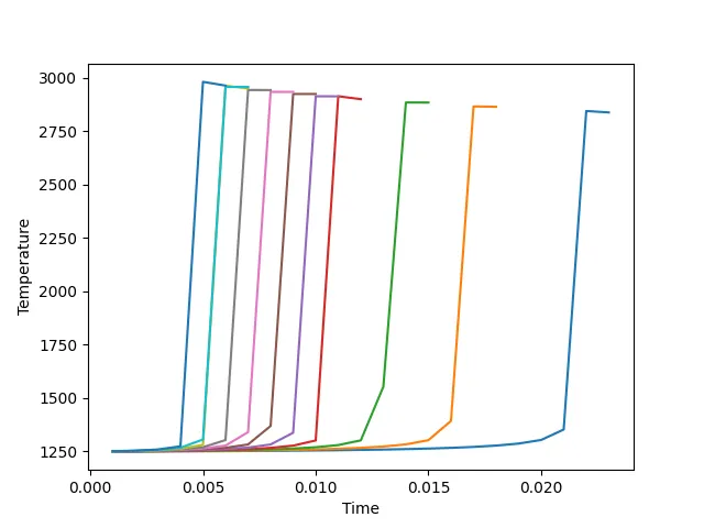
The above graph depicts that, the temperature change is constant for different time scales. At initial time temperature change linearly but, as time increases temperature change logarithmically due to delay time. From the above figure, we can analyze that due to a very small delay time temperature change remains constant. From left to right temperature delay time increases linearly.

PART-B

In this case, further observe and print the rate of change of molar concentrations of the given elements H2O, O2 & OH with respect to the time (i.e. simulation time = 10 secs).

CH4 + 2(O2 + 7.52N2) = CO2 + 2H2O + 7.52N2

CASE-1:-

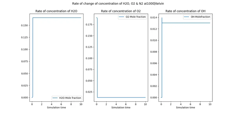
In this case, calculate the molar fraction of product species using Cantera.

In the above figure, we can see that the rate of the molar fraction of H2O, O2 & OH at 1000k.

The first plot tells the mole fraction of H2O it is respectively very less before auto-ignition. As we discussed before the reaction of methane and air forms the product of H2O and it's starting very little after ignition takes place it becomes increases and somewhere it's getting to stability this is called equilibrium chemistry.

The second plot is to define the mole fraction of O2 it respectively decreases because it is air and reacts with fuel and gets oxidized.

The third plot tells the mole fraction of OH it is respectively very less before auto-ignition. As we discussed before the reaction of methane and air it forms the product of OH and it's starting very less after ignition takes place it becomes increases and somewhere it's getting to stability this is called equilibrium chemistry.

• In the first case, the H2O mole fraction is maximum at the start but it remains constant at peak point for all simulation time.
• In the second case, the O2 mole fraction minimum at the start but it remains constant at the lowest point for all simulation time.
• In the third case, the OH mole fraction is maximum at the start and later on remains constant just below the peak point of the start for all simulation time.

CASE-2:-

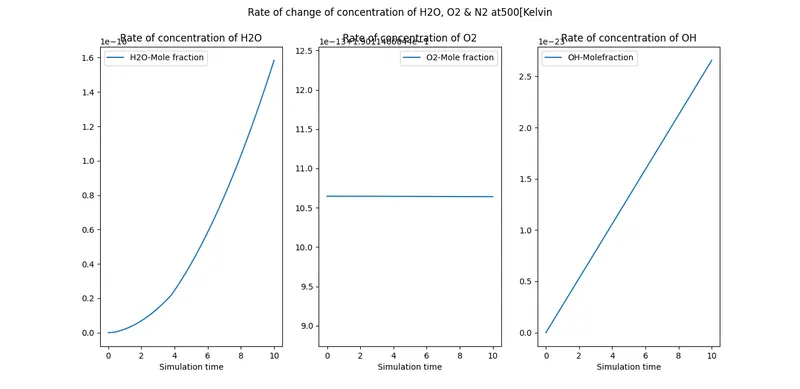
In this case, the calculated molar fraction of H2O, O2, and OH at 500k, the rate mole fraction is very less as compared to the 1000k because the initial temperature was very low. In the first plot we see that very slowly auto-ignition takes place and the second plot 'O2' Is not completely atomize because the initial temperature was very low.

• In the first case, the H2O mole fraction increases parabolically from zero to 1.6 for all simulation time.
• In the second case, the O2 mole fraction remains constant at 10.7 for all simulation time.
• In the third case, the OH mole fraction increases linearly from zero to 2.7 for all simulation time.

CONCLUSIONS:-

From the above code and its results, we can conclude the following points i.e. ignition delay.

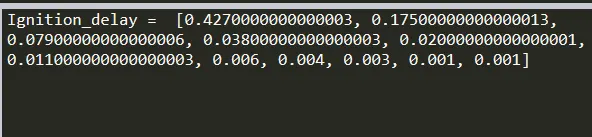
1. Ignition delay for constant pressure:-

2. Ignition delay for constant temperature:-

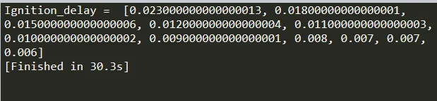
From the above output, we can clearly analyze that ignition delay decreases as temperature or pressure increases and vice versa.

• Ignition delay is maximum for constant pressure and it decreases fastly.
• Ignition delay is comparatively lower for constant temperature and it decreases slowly.
• Ignition delay occurs due to temperature or pressure difference also incomplete burning of an air-fuel mixture or leans or rich mixture.