Week 7 - Auto ignition using Cantera
AUTO-IGNITION USING CANTERA
Objective: To simulate the Auto Ignition Time for Methane under certain conditions and also observe the rate of change of molar concentrations of some elements.
Introduction: The auto-ignition temperature of a substance is the lowest temperature in which it spontaneously ignites in a normal atmosphere without an external source of ignition, such as a flame or spark.
Part-1: Simulating the Auto Ignition Time for Methane under the following conditions, (simulation time = 10 secs).
`CH_4 + 2(O_2 + 3.76N_2) = CO_2 + 2H_2O + 7.52N_2`
Case-1: Plot the variation of Auto Ignition time of Methane with a constant temperature of 1250K and pressure varying from 1 to 5 atm.
'''
Plot the variation of Auto Ignition time using Reactor and ReactorNet Using Cantera of Methane
with a constant temperature of 1250K and pressure varying from 1 to 5 atm.

Reaction:

CH4 + 2(O2 + 3.76N2) = CO2 + 2H2O + 7.52N2

'''

import sys
import cantera as ct
import matplotlib.pyplot as plt
import numpy as np

gas = ct.Solution('gri30.xml')
ignition_delay=[]
pressure = np.linspace(1,5,5)#pressure = 1 t0 5 atms.

for p in pressure:

	T=1250 # Temperature
	gas.TPX = T,ct.one_atm*p,{'CH4':1,'O2':2,'N2':7.52}
	r = ct.IdealGasReactor(gas)
	sim = ct.ReactorNet([r])
	time = 0.0
	states = ct.SolutionArray(gas,extra=['time_in_ms','t'])
	T_o = T
	# Time loop
	for j in range(10000): # time = 10sec
		time += 1e-3
		sim.advance(time) # Time step
		states.append(r.thermo.state,time_in_ms = time*1e-3,t = time)
		T_p = states.T# temperature at different pressure
		T_p = T_p[j-1]

		if (T_p-T_o)>=400:# ignition delay calculation
			ignition_delay.append(time)
		T_o = states.T
		T_o = T_o[j-1]

	plt.subplot(2,1,1)
	plt.plot(states.t,states.T)
	plt.xlabel('Simulation time (ms)')
	plt.ylabel('Temprature(k)')
	plt.legend(['Pressure -'+str(p)+'[atm]'for p in pressure])
	plt.title('Effect of pressure on final temperature')


plt.subplot(2,1,2)
plt.plot(pressure,ignition_delay,'-o')
plt.xlabel('Pressure')
plt.ylabel('ignition_delay')
plt.show()
Results:
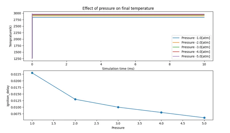
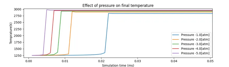
- From the above graphs, it can be observed that Rise in the pressure of the reaction chamber where combustion due to auto-ignition takes place helps in less ignition delay and vice-versa.
Case-2: Plot the variation of Auto Ignition time of Methane with a constant pressure of 5 atm and temperature varying from 950K to 1450K.
'''
Plot the variation of Auto Ignition time using Reactor and ReactorNet Using Cantera of Methane with
a constant pressure of 5atm and temperature varying from 950K to 1450K.

Reaction:

CH4 + 2(O2 + 3.76N2) = CO2 + 2H2O + 7.52N2

'''

import sys
import cantera as ct
import matplotlib.pyplot as plt
import numpy as np

gas = ct.Solution('gri30.xml')
ignition_delay=[]
Temp = np.linspace(950,1450,5)
for T in Temp:

	P = 5 #atm pressure
	gas.TPX = T,ct.one_atm*P,{'CH4':1,'O2':2,'N2':7.52}
	r = ct.IdealGasReactor(gas)
	sim = ct.ReactorNet([r])
	time = 0.0
	states = ct.SolutionArray(gas,extra=['time_in_ms','t'])
	T_o = T

	# Time loop
	for j in range(10000): # time = 10sec.
		time += 1e-3
		sim.advance(time) # Time step
		states.append(r.thermo.state,time_in_ms = time*1e-3,t = time)
		T_p = states.T
		T_p = T_p[j-1]

		if (T_p-T_o)>=400:# ignition delay calculation
			ignition_delay.append(time)
		T_o = states.T
		T_o = T_o[j-1]

	plt.subplot(2,1,1)
	plt.plot(states.t,states.T)
	plt.xlabel('Simulation time (ms)')
	plt.ylabel('Temperature(k)')
	plt.legend(['Temperature -'+str(T)+'K'for T in Temp])
	plt.title('Effect of pressure on final temperature')

plt.subplot(2,1,2)
plt.plot(Temp,ignition_delay,'-o')
plt.xlabel('Temperature')
plt.ylabel('ignition_delay')
plt.show()
Results:
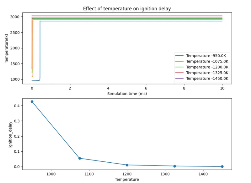
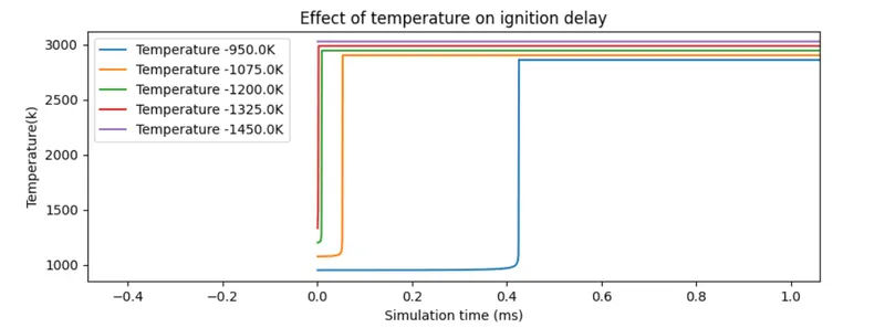
- Higher temperature means faster reactions and faster auto-ignition which results in the less ignition delay.
- At 1450k, Auto ignition taken place immidiatly. Combustion taken place at a micro second scale.
Part-2: Rate of change of molar concentrations of the given elements "H2O, O2, OH" with respect to the time, (simulation time = 10 secs)
#Rate of change of molar concentrations of the given elements "H2O, O2, OH" with respect to the time, (simulation time = 10 secs).

import sys
import cantera as ct
import matplotlib.pyplot as plt
import numpy as np

gas = ct.Solution('gri30.xml')
ignition_delay=[]
Temp = [1000, 500]

for T in Temp:
	P = 5 #atm pressure
	gas.TPX = T,ct.one_atm*P,{'CH4':1,'O2':2,'N2':7.52}
	r = ct.IdealGasReactor(gas)
	sim = ct.ReactorNet([r])
	time = 0.0
	states = ct.SolutionArray(gas,extra=['time_in_ms','t'])
	# Time loop
	for j in range(10000): # time = 10sec.
		time += 1e-3
		sim.advance(time) # Time step
		states.append(r.thermo.state,time_in_ms = time*1e-3,t = time)

	plt.subplot(3,1,1)
	plt.plot(states.t,states.X[:,gas.species_index('H2O')])
	plt.xlabel('Time [ms]')
	plt.ylabel('H2O')
	plt.title('Molar concentrations of species w.r.t time at temperature:'+str(T))

	plt.subplot(3,1,2)
	plt.plot(states.t,states.X[:,gas.species_index('O2')])
	plt.xlabel('Time [ms]')
	plt.ylabel('O2')

	plt.subplot(3,1,3)
	plt.plot(states.t,states.X[:,gas.species_index('OH')])
	plt.xlabel('Time [ms]')
	plt.ylabel('OH')
	plt.show()
Case-1: When Temperature is 1000K and pressure 5 bar
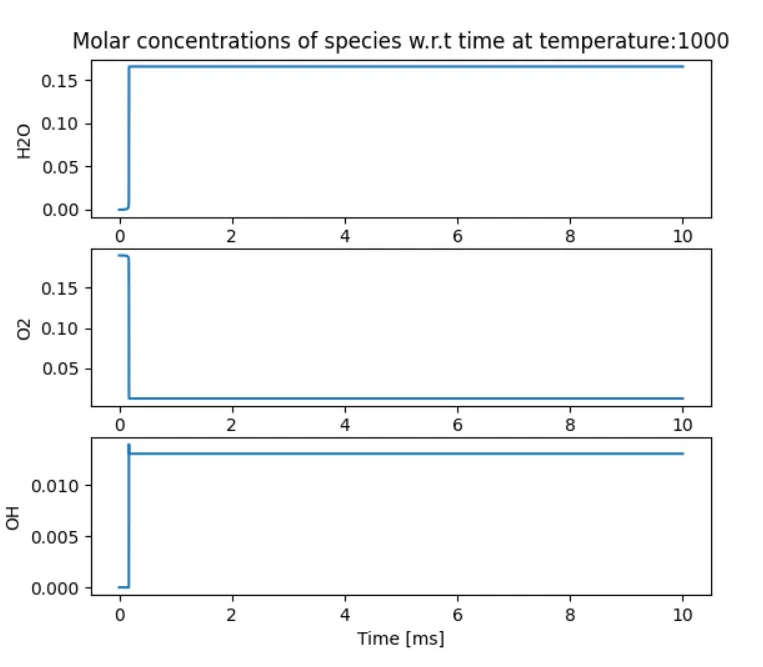
- H2O formed due to the combustion process. Its concentration remained constant after the combustion taken place.
- O2 is oxidizer of the fuel in this reaction. Once the auto-ignition taken place its concentration decreased as oxygen molecules got seperated to form other species.
- Like H20, OH also formed due to the combustion.
case-2: When Temperature is 500K and pressure 5 bar
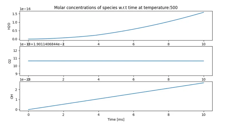
- Compared to the concentrations of the above graph, we can observe that their is a peculiar behaviour in the concentration of the species at temperature 500 kelvin.
- To understand this behaviour, We must know the auto-ignition temperature of the methane which is around = 600C or 873 kelvin. Which means the auto ignition did not take place that is no combustion.
- However Concentrations of H2O and OH changed due to reactions that have taken place in ambient temperature. Where as the O2 concentration remained constant due to no combustion.