Auto ignition simulation using Cantera

AIM –

1. To simulate auto ignition in a methane air mixture using Cantera in Python interface.
2. Study the effect of initial temperature and pressure on the ignition delay in the same mixture.
3. Study the effect of temperature on molar concentration of H2O, O2 and OH in the same system at 5 atm.

THEORY -

Auto ignition occurs when a mixture of gases or vapors ignites spontaneously with no external ignition source and after reaching a certain temperature, the auto ignition temperature. The auto ignition temperature is not an intrinsic property of the gases or vapors but is the lowest temperature in a system where the rate of heat evolved from the gases or vapors increases beyond the rate of heat loss to the surroundings, resulting in ignition. The auto ignition temperature of a mixture of gases or vapors is affected by pressure, vessel shape and volume, surface activity, contaminants, flow rate, reaction rate, droplet and mist formation, gravity, and reactant concentration.

To simulate the auto ignition phenomenon in a methane air mixture, Cantera has been used in Python.

Simulating 0D chemical systems in Cantera –

A system in which the properties have no gradients along any direction is called a 0D reacting system. This is the simplest form of reacting system, and a small closed cylinder can be thought of a 0D reactor.

Different types of reactors (as classes) are available in Cantera –

1. Reservoir - A reservoir is a reactor with a constant state. The temperature, pressure, and chemical composition in a reservoir never change from their initial values.
2. Reactor – It is a homogeneous zero-dimensional reactor. By default, they are closed (no inlets or outlets), have fixed volume, and have adiabatic, chemically-inert walls. These properties may all be changed by adding appropriate components, e.g. Wall, MassFlowController and Valve.
3. IdealGasReactor - A constant volume, zero-dimensional reactor for ideal gas mixtures.
4. ConstPressureReactor - A homogeneous, constant pressure, zero-dimensional reactor. The volume of the reactor changes as a function of time in order to keep the pressure constant.
5. IdealGasConstPressureReactor - A homogeneous, constant pressure, zero-dimensional reactor for ideal gas mixtures. The volume of the reactor changes as a function of time in order to keep the pressure constant.
6. FlowReactor - A steady-state plug flow reactor with constant cross sectional area. Time integration follows a fluid element along the length of the reactor. The reactor is assumed to be frictionless and adiabatic.

Reactors can interact with the surrounding environment in multiple ways:

• Expansion/compression work: By moving the walls of the reactor, its volume can be changed and expansion or compression work can be done by or on the reactor.
• Heat transfer: An arbitrary heat transfer rate can be defined to cross the boundaries of the reactor.
• Mass transfer: The reactor can have multiple inlets and outlets. For the inlets, arbitrary states can be defined. Fluid with the current state of the reactor exits the reactor at the outlets.
• Surface interaction: One or multiple walls can influence the chemical reactions in the reactor. This is not just restricted to catalytic reactions, but mass transfer between the surface and the fluid can also be modeled.

In this study, we simulate a simple batch reactor at constant volume (a rigid vessel with constant volume). Therefore, IdealGasReactor (without any interaction with the surroundings) class is our choice.

Governing Equations for single reactors –

The state variables for Cantera’s general reactor model are

• m, the mass of the reactor’s contents (in kg)
• V, the reactor volume (in m³) (not a state variable for ConstPressureReactor() and IdealGasConstPressureReactor())
• A state variable describing the energy of the system, depending on the configuration-
  • Reactor(): U, the total internal energy of the reactors contents (in J)
  • ConstPressureReactor(): H, the total enthalpy of the reactors contents (in J)
  • IdealGasReactor() and IdealGasConstPressureReactor(): T, the temperature (in K)
• Y_k​, the mass fractions for each species (dimensionless)

Mass Conservation

The total mass of the reactor’s contents changes as a result of flow through the reactor’s inlets and outlets, and production of homogeneous phase species on the reactor walls:

`(dm)/dt=underset(i)Sigmadotm_(i) - underset(o)Sigmadotm_(o) + dotm_(wall)`

Species Conservation

The rate at which a homogenous species k is generated through homogeneous phase reactions is `Vdot(omega)_kW_k` and the total rate at which species k is generated is –

`dot m_k = Vdotω_k W_k + dotm_(wall)`

The rate of change of mass of each species is

`(dmY_k )/dt=underset(i)Sigmadotm_(i)Y_(k,i) - underset(o)Sigmadotm_(o)Y_(k,o) + dotm_(k,Gen)`

Expanding the derivative on the LHS and substituting the value of dm/dt –

`m(dY_k )/dt=underset(i)Sigmadotm_(i)(Y_(k,i)-Y_(k,o)) + dotm_(k,Gen)-Y_kdotm_(k,wall)`

Reactor Volume

The reactor volume changes as a function of time due to the motion of one or more walls:

`(dV)/dt= underset(w)∑f_w A_w v_w (t)`

where `f_w = +-1` indicates the facing of the wall (whether moving the wall increases or decreases the volume of the reactor), `A_w` is the surface area of the wall, and `v_w (t)` is the velocity of the wall as a function of time.

For the ConstPressureReactor() and IdealGasConstPressureReactor(), the volume is not a state variable, but instead takes on whatever value is consistent with holding the pressure constant.

Energy Conservation

The solution of the energy equation can be enabled or disabled by changing the energy_enabled flag. It is enabled by default.

The implemented formulation of the energy equation depends on which reactor model is used.

In case of the Ideal Gas Reactor Model, the reactor temperature T is used instead of the total internal energy U as a state variable.

Reactor Networks and Devices –

While reactors by themselves just define the above governing equations of the reactor, the time integration is performed in reactor networks. A reactor network is therefore necessary even if only a single reactor is considered.

The advantage of reactor networks obviously is that multiple reactors can be interconnected. Not only mass flow from one reactor into another can be realized, but also heat can be transferred, or the wall between reactors can move. To set up a network, the following components can be defined in addition to the reactors previously mentioned:

• Reservoir(): A reservoir can be thought of as an infinitely large volume, in which all states are predefined and never change from their initial values. Typically, it represents a vessel to define temperature and composition of a stream of mass flowing into a reactor, or the ambient fluid surrounding the reactor network. Besides, the fluid flow finally finally exiting a reactor network has to flow into a reservoir. In the latter case, the state of the reservoir (except pressure) is irrelevant.
• Wall(): A wall separates two reactors, or a reactor and a reservoir. A wall has a finite area, may conduct or radiate heat between the two reactors on either side, and may move like a piston.
• Valve(): A valve is a flow devices with mass flow rate that is a function of the pressure drop across it. The default behavior is linear.

Time integration –

Cantera provides an ODE solver for solving the stiff equations of reacting systems. If Cantera is installed with SUNDIALS (the default), the optimized solver from SUNDIALS is used. Starting off the current state of the system, it can be advanced in time by one of the following methods:

• step(): The step method computes the state of the system at the a priori unspecified time t_new. The time t_new is internally computed so that all states of the system only change within a (specifiable) band of absolute and relative tolerances. Additionally, the time step must not be larger than a predefined maximum time step ∆t_max. The new time t_new is returned by this function.
• advance(t_new ​): This method computes the state of the system at time t_new. t_new ​ describes the absolute time from the initial time of the system. By calling this method in a for loop for pre-defined times, the state of the system is obtained for exactly the times specified. Internally, several step()calls are typically performed to reach the accurate state at time t_new.
• advance_to_steady_state(max_steps, residual_threshold, atol, write_residuals)[Python interface only]: If the steady state solution of a reactor network is of interest, this method can be used. Internally, the steady state is approached by time stepping. The network is considered to be at steady state if the feature-scaled residual of the state vector is below a given threshold value (which by default is 10 times the time step rtol).

The use of the advance method in a loop has the advantage that it produces results corresponding to a predefined time series. These are associated with a predefined memory consumption and well comparable between simulation runs with different parameters. However, some detail (for example, a fast ignition process) might not be resolved in the output data due to the typically large time steps.

The step method results in much more data points because of the small time steps needed. Additionally, the absolute time has to be kept track of manually.

Even though Cantera comes pre-defined with typical parameters for tolerances and the maximum internal time step, the solution sometimes diverges. To solve this problem, three parameters can be tuned: The absolute time stepping tolerances, the relative time stepping tolerances, and the maximum time step. A reduction of the latter value is particularly useful when dealing with abrupt changes in the boundary conditions (for example, opening/closing valves).

General Usage in Cantera

In Cantera, the following steps are typically necessary to investigate a reactor network:

1. Define Solutionobjects for the fluids to be flowing through your reactor network.
2. Define the reactor type(s) and reservoir(s) that describe your system. Chose Ideal Gas (Constant Pressure) Reactor(s) if you only consider ideal gas phases.
3. Optional:Set up the boundary conditions and flow devices between reactors or reservoirs.
4. Define a reactor network which contains all the reactors previously created.
5. Advance the simulation in time, typically in a for- or while-loop. Note that only the current state is stored in Cantera by default. If you want to observe the transient states, you manually have to keep track of them.
6. Analyze the data.

Note that Cantera always solves a transient problem. If you are interested in steady-state conditions, you can run your simulation for a long time until the states are converged.

Solution Algorithm –

1. Initialize a gas object from the Solution class. GRI30.xml can be used as the reaction mechanism file for input. Also initialize the total time of simulation.
2. Set the initial temperature, pressure and species mole fraction of the gas object.
3. Create a new object, say r, from the IdealGasReactor class of Cantera.
4. Use r as an input to the ReactorNet class and create a reactor network, say sim.
5. Advance the sim object by 1 millisecond (ms) for the total simulation time.
6. Append the thermal properties after each millisecond. For this, use the SolutionArray class for proper formatting of data.
7. To calculate the ignition delay, store the time at which the difference in the initial temperature and the current temperature of the reactor is 400 K.
8. Repeat the above steps for either different temperatures or different pressures.

Results and Discussions –

Auto Ignition and Ignition delay time at different temperatures and pressures –

It can be inferred from the below graphs that ignition delay is a strong function of ambient pressure and temperature. The value ignition delay for different ambient conditions is given in the below table-

Initial Pressure (atm), T = 1250 K	Ignition Delay (ms)
1	22
2	12
3	9
4	7
5	5

Initial Temperature (K), P = 1 atm	Ignition Delay (ms)
950	2654
1050	450
1150	91
1250	21
1350	6
1450	2

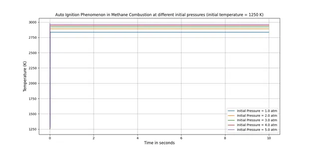
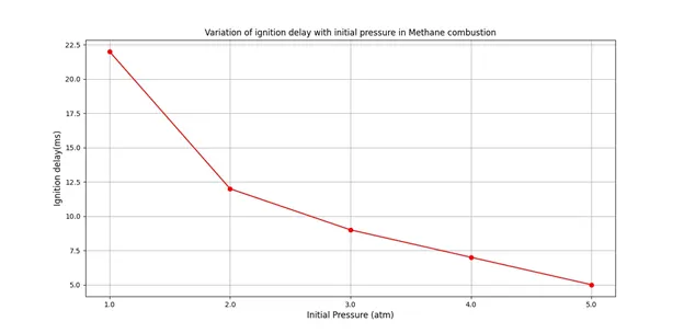
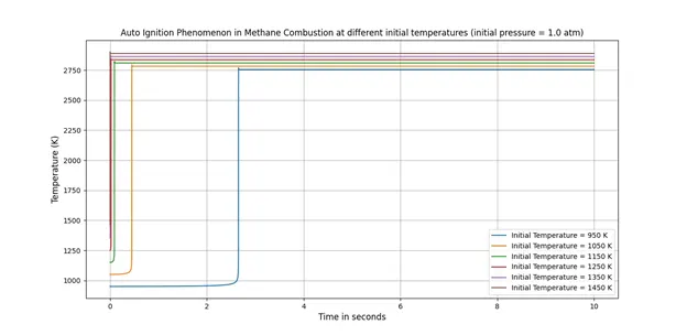
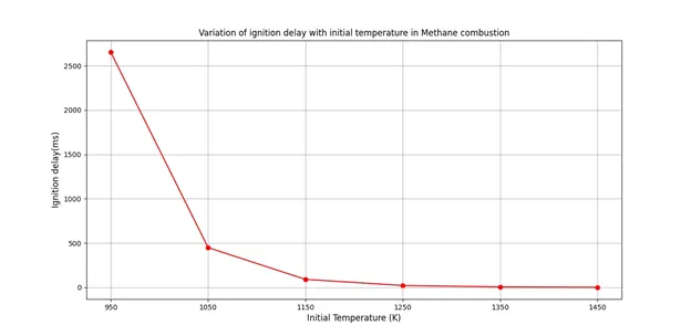
This can be attributed to the fact that the chemical kinetics speed up as the pressure or temperatures are increased. The physical and chemical delays of the reactions decrease with increase in ambient temperatures and pressures. This, therefore, leads to lower ignition delays. The ignition delay is significantly high at 950 K because the temperature is very near to the ignition temperature of methane (870 K at 1 atm).

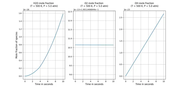
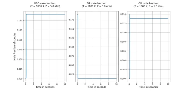
To extend this study, molar concentrations of H2O, O2 and OH have been observed at 1000 K and 500 K, keeping the ambient pressure as 5 atm. It was observed that at temperature of 1000 K the mixture auto ignites as indicated by the decrease in molar concentration of O2 and increase in the concentration of H2O and OH. However, at 500 K , there is no auto ignition due to the low temperature. There is still some variation in the mole fraction of H2O and OH because of their formation in other elementary reactions which take place as indicated in the GRI 3.0 Mechanism.

PYTHON CODE FOR AUTO IGNITION AND IGNITION DELAY -

import math
import numpy as np 
import matplotlib.pyplot as plt 
import cantera as ct

gas = ct.Solution('gri30.xml')
T = [950,1050,1150,1250,1350,1450]	#Initial temperature in Kelvin
# T = 1250
P_atm = 101325 	#AtmosphericPressure in Pascal
# mult_list = [1,2,3,4,5]
# P = [x*P_atm for x in mult_list]
P = P_atm
phi = 1
species_dict = {'CH4':1,'O2':2/phi,'N2':3.76*2/phi}	#Species moles in the reactor. Moles of each species on 
#reactant side written in terms of phi. Can also be written as mole fractiom
ig_delay = []
t_end = 10*1000	#in milliseconds

for i in range(len(T)):
	ig_ctr = 0
	#T_new = 0
	gas.TPX = T[i],P,species_dict
	# gas.TPX = T,P[i],species_dict
	r = ct.IdealGasReactor(gas) #Object created from the ideal gas reactor class of cantera
	sim = ct.ReactorNet([r])	#Object created from the reactor newtork class of cantera. Helps in advancing the states at each time step
	time = 0.0
	states = ct.SolutionArray(gas,extra = ['time_in_ms','t'])
	# T_old = T
	T_old = T[i]
	k=0

	for t in range(t_end):
		time+=0.001	#Upper limit of integration. It is not the time step size. 
		sim.advance(time)	#Advance method in the reactorNet class advances the states at each time
		states.append(r.thermo.state,time_in_ms = time*1e3,t=time)
		if(k==0):
			T_new = states.T
			T_new = T_new[t]
			
			if ((T_new-T_old)>=400 and ig_ctr == 0):
				ig_delay.append(states.time_in_ms[t])
				ig_ctr = ig_ctr+1
				k=k+1
	
	plt.figure(1)
	plt.plot(states.t,states.T)

#Plotting.
plt.xlabel('Time in seconds',fontsize = 12)
plt.ylabel('Temperature (K)',fontsize = 12)
# plt.legend(['Initial Pressure = '+str(i/P_atm)+' atm' for i in P])
plt.legend(['Initial Temperature = '+str(i)+' K' for i in T])

# plt.title('Auto Ignition Phenomenon in Methane Combustion at different initial pressures (initial temperature = {0} K)'.format(T))
plt.title('Auto Ignition Phenomenon in Methane Combustion at different initial temperatures (initial pressure = {0} atm)'.format(P/P_atm))
plt.grid('on')

plt.figure(2)
# plt.plot(P,ig_delay,'ro-')
plt.plot(T,ig_delay,'ro-')
print(ig_delay)
# plt.xlabel('Initial Pressure (atm)',fontsize = 12)
plt.xlabel('Initial Temperature (K)',fontsize = 12)
# xt = [j/P_atm for j in P]
# plt.xticks(P,xt)
xt = [j for j in T]
plt.xticks(T,xt)
plt.ylabel('Ignition delay(ms)',fontsize = 12)
# plt.title('Variation of ignition delay with initial pressure in Methane combustion')
plt.title('Variation of ignition delay with initial temperature in Methane combustion')

plt.grid('on')

plt.show()

PYTHON CODE FOR MOLAR CONCENTRATIONS

import math
import numpy as np 
import matplotlib.pyplot as plt 
import cantera as ct

gas = ct.Solution('gri30.xml')
T = [500,1000]	#Initial temperature in Kelvin
P_atm = 101325 	#AtmosphericPressure in Pascal
P = 5*P_atm
phi = 1
species_dict = {'CH4':1,'O2':2/phi,'N2':3.76*2/phi}	#Species moles in the reactor. Moles of each species on 
#reactant side written in terms of phi. Can also be written as mole fractiom
t_end = 10*1000	#in milliseconds

for i in range(len(T)):
	gas.TPX = T[i],P,species_dict
	r = ct.IdealGasReactor(gas) #Object created from the ideal gas reactor class of cantera
	sim = ct.ReactorNet([r])	#Object created from the reactor newtork class of cantera. Helps in advancing the states at each time step
	states = ct.SolutionArray(gas,extra = ['time_in_ms','t'])
	time = 0.0
	for t in range(t_end):
		time+=0.001	#Upper limit of integration. It is not the time step size. 
		sim.advance(time)	#Advance method in the reactorNet class advances the states at each time
		states.append(r.thermo.state,time_in_ms = time*1e3,t=time)

	#Plotting.
	plt.figure(i+1)
	plt.subplot(131)
	plt.plot(states.t,states.X[:,gas.species_index('H2O')])
	plt.grid('on')
	plt.xlabel('Time in seconds',fontsize = 12)
	plt.ylabel('Mole Fraction of species',fontsize = 12)
	plt.title('H2O mole fraction n(T = {0} K, P = {1} atm)n'.format(T[i],P/P_atm))
	plt.subplot(132)
	plt.plot(states.t,states.X[:,gas.species_index('O2')])
	plt.grid('on')
	plt.xlabel('Time in seconds',fontsize = 12)
	plt.title('O2 mole fraction n(T = {0} K, P = {1} atm)n'.format(T[i],P/P_atm))
	plt.subplot(133)
	plt.plot(states.t,states.X[:,gas.species_index('OH')])
	plt.grid('on')
	plt.xlabel('Time in seconds',fontsize = 12)
	plt.title('OH mole fraction n(T = {0} K, P = {1} atm)n'.format(T[i],P/P_atm))

plt.show()