Week-6 : Turbocharger Modelling

Turbocharger Modelling

Objectives:

• Explore the steps in modeling a 6 cylinder DI Turbocharged Engine (Tutorial 6cylDIturbo and Turbocharging in GT Suite)
• Explore the steps to build an Engine with VGT EGR (Example Diesel VGT EGR in GT Suite)

Turbocharger:

Turbocharger is a compressor and turbine coupled system to increase charge air pressure.

They are of different types based on the feature it provides

• Single Turbo

Single turbochargers are what most people think of as turbos. By differing the size of the elements within the turbo, completely different torque characteristics can be achieved. Large turbos provide higher levels of top end power, whilst smaller turbos can spool faster and provide better low-end power. They are a cost-effective way of increasing engine power and efficiency, and as such have become increasingly popular, allowing smaller engines to increase efficiency by producing the same power as larger naturally-aspirated engines, but with a lower weight. They do however tend to work best within a narrow RPM range, and drivers will often experience ‘turbo-lag’ until the turbo starts to operate within its peak rev band.

• Twin Turbo

• Twin Scroll Turbo

Twin-scroll turbochargers require a divided-inlet turbine housing and exhaust manifold that pairs the correct engine cylinders with each scroll. independently. For example, in a four-cylinder engine (with a firing order 1-3-4-2), cylinders 1 and 4 might feed to one scroll of the turbo, while cylinders 2 and 3 feed to a separate scroll. This layout provides more efficient delivery of exhaust gas energy to the turbo, and results and helps provide denser, purer air into each cylinder. More energy is sent to the exhaust turbine, meaning more power. Again, there is a cost penalty for addressing the complexity of a system requiring complicated turbine housings, exhaust manifolds and turbos. Example: Diesel_6cyl_TC

Example: Diesel_6cyl_TC

• VGT (Variable Geometry Turbocharger)

Typically, VGTs include a ring of aerodynamically-shaped vanes in the turbine housing at the turbine inlet. In turbos for passenger cars and light commercial vehicles, these vanes rotate to vary the gas swirl angle and the cross-sectional area. These internal vanes alter the turbos area-to-radius (A/R) ratio to match the engines RPM, and so give peak performance. At low RPM, a low A/R ratio allows the turbo to quickly spool up by increasing exhaust gas velocity and. At higher revs the A/R ratio increases, thereby allowing increased airflow. This results in a low boost threshold reducing turbo lag, and provides a wide and smooth torque band. Whilst VGTs are more typically used in diesel engines where exhaust gases are lower temperature, until now VGTs have been limited in petrol engine applications due to their cost and the requirement for components to be made from exotic materials. The high temperature of the exhaust gases means that the vanes must be made from exotic heat-resistant materials to prevent damage. This has restricted their use to applications within luxury, high performance engines. The variable geometry turbine allows significant flexibility over the pressure ratio across the turbine. In diesel engines, this flexibility can be used for improving low speed torque characteristics, reducing turbocharger lag and driving EGR flow.

Example: Diesel VGT EGR

Example: Diesel VGT EGR

• Variable Twin Scroll Turbo

As the name suggests a VTS turbocharger combines the advantages of a twin-scroll turbo and a variable geometry turbo. It does this by the use of a valve which can redirect the exhaust airflow to just a single scroll, or by varying the amount the valve opens can allow for the exhaust gases to split to both scrolls. The VTS turbocharger design provides a cheaper and more robust alternative to VGT turbos, meaning it is a viable option for petrol engine applications

• WGT (Waste Gate Turbocharger)

Nowadays, vehicles with turbocharged engines feature the wastegate turbocharger. This technology helps to deliver optimum engine performance during peak operating conditions. In addition, the wastegate valve prevents the turbocharger from over-running. Particularly, it also avoids the engine from over-boost and prevents any mechanical failure.This feature in the turbocharger consists of a bypass valve. It circumvents some part of the exhaust gas going to the turbine and releases them into the outlet. Furthermore, the waste-gate turbocharger has a bypass valve built into the turbine housing. It diverts some of the exhaust gases away from the turbine wheel through this valve.

Example: Diesel_WGController

• Electric turbocharger

An electric turbocharger is used to eliminate turbo lag and assist a normal turbocharger at lower engine speeds where a conventional turbo is not most efficient. This is achieved by adding an electric motor that spins up the turbo’s compressor from start and through the lower revs, until the power from the exhaust volume is high enough to work the turbocharger. This approach makes turbo lag a thing of the past, and significantly increases the RPM band within which the turbo will efficiently operate. So far, so good. It appears that electronic turbos are the answer to all the negative characteristics of conventional turbochargers, however there are some disadvantages. Most are around cost and complexity, as the electric motor must be accommodated and powered, plus also cooled to prevent reliability issues.

PART 1

Single Cylinder DI Engine:

Lets convert a Single Cylinder DI Engine into a 6 Cylinder DI Engine with Turbocharger.

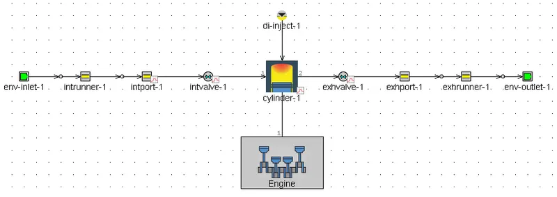
Base Engine Modelling:

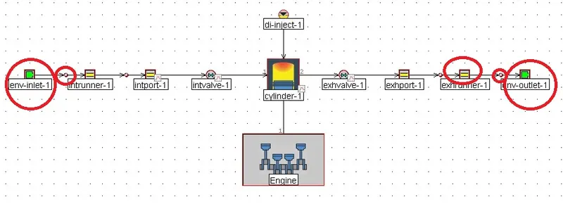
Step 1: Delete the inlet end environment, orifice connection 1, the exhaust runner, orifice connection 4, and the outlet end environment. Delete the direct connection between the cylinder and EngineCrankTrain.

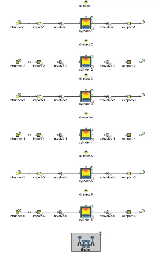
Step 2: 6 Copies of the same modified model is made in order to build a 6 cylinder Engine.

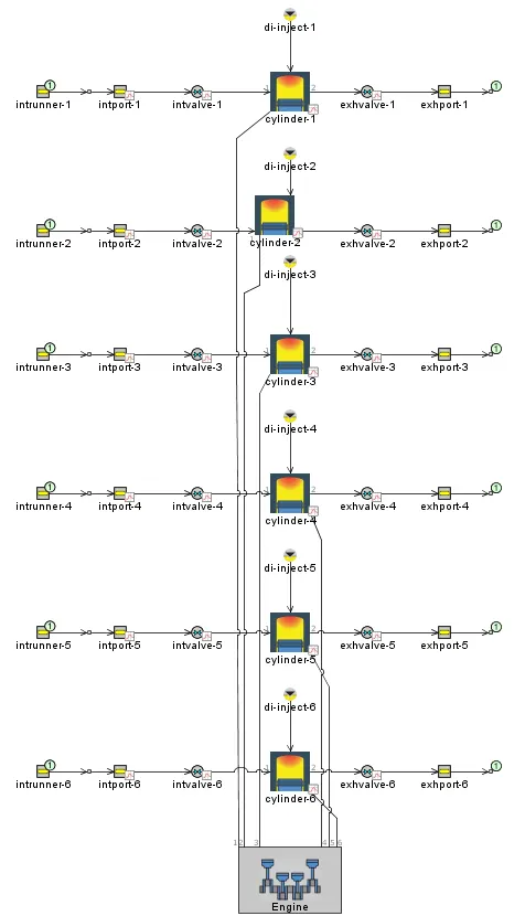
Step 3: Firing order is set to 1-5-3-6-2-4 in Engine Cranktrain object.

Step 4: Create a link between cylinders and Engine Cranktrain.

Intake System Modelling-Intercooler:

The intake system will consist of an intercooler (aftercooler, charge air cooler) and a log-style intake manifold. The six intake runners for the cylinders will connect the manifold to the intake ports.

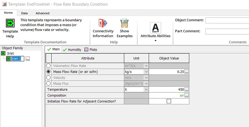
Step 5: EndflowInlet object is assigned with a name of inlet 1 with mass flow rate of 0.25 kg/s, Temperature 450K and air as the working fluid.

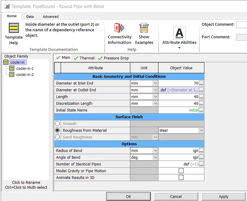
Step 6: Cooler inlet is defined using the PipeRound object with a diameter of 70mm,length 40mm and steel as its object.

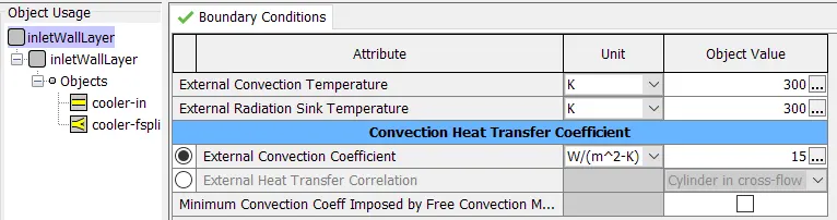
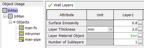
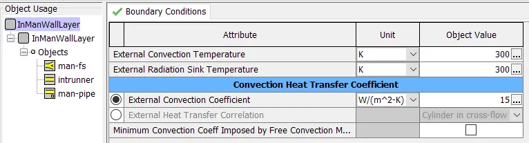
• Initial wall temperature is assigned to be at 350K and Wall Layer Properties and External Boundary Conditions are defined as separate objects.

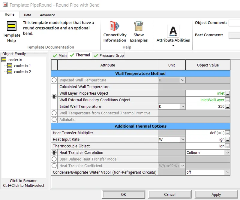
• Inlet Object is assigned to Wall properties object with the following properties.

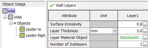
• inletWallLayer Object is assigned to Wall External Boundaries object with the following properties.

Step 7: Cooler Flow Splits at upstream and downstream are defined.

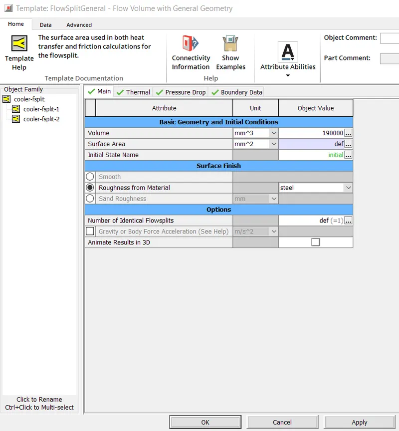
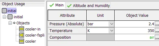
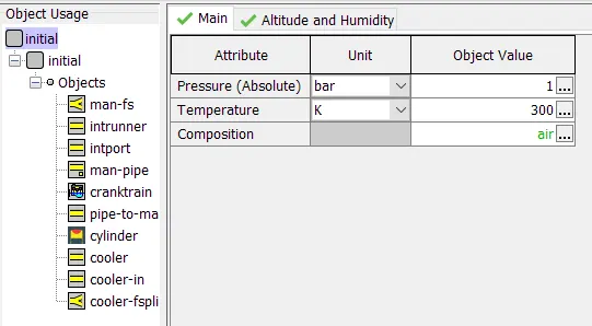
• initial state object is defined using below variables.

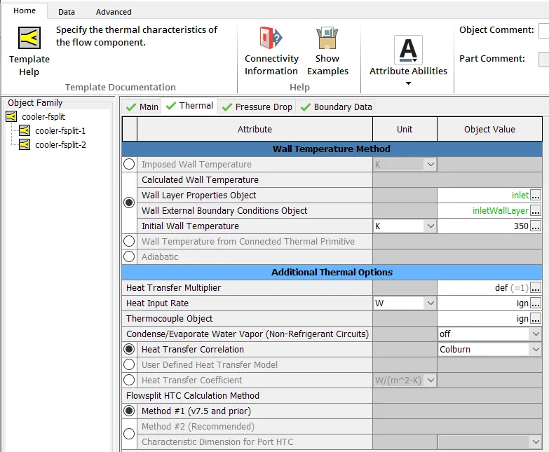
• Thermal conditions are imposed as same as before in case of coolent inlet.

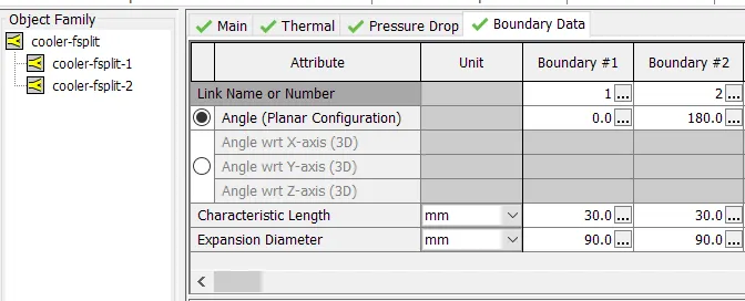
• Boundary data regarding the splitting of cooler geometry is defined as follows.

Step 8: Defining intercooler data.

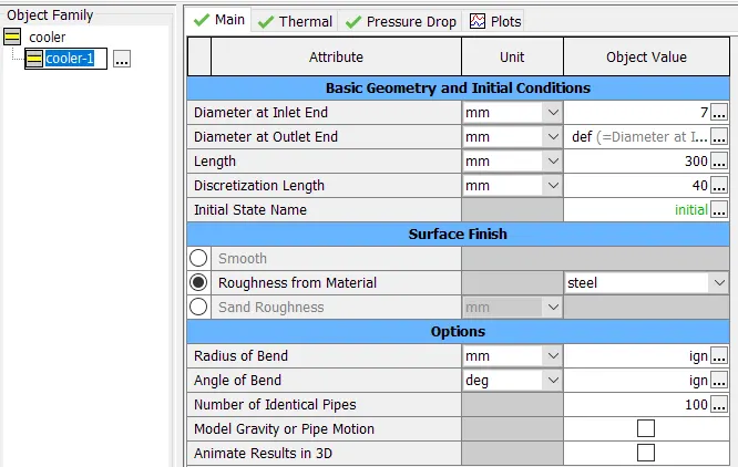
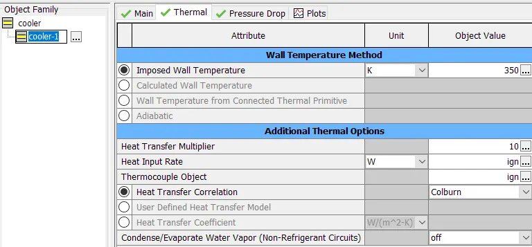
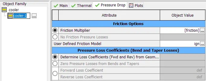
• Under Pressure Drop data, Friction Multiplier is made as a user defined object which can be tuned further to optimize the results from intercooler. By default it is set to 1.

Step 9: EndEnvironment is the final output from the intercooler. It is defined with the below parameters.

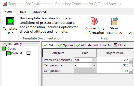
Step 10: Intercooler Effectiveness

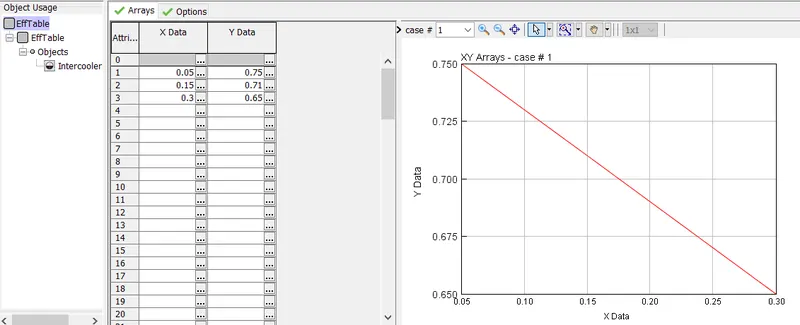
• This template will use an effectiveness table as input, which is typically available from the supplier of the cooler. It will impose a cooler effectiveness over air mass flow at a given coolant temperature.
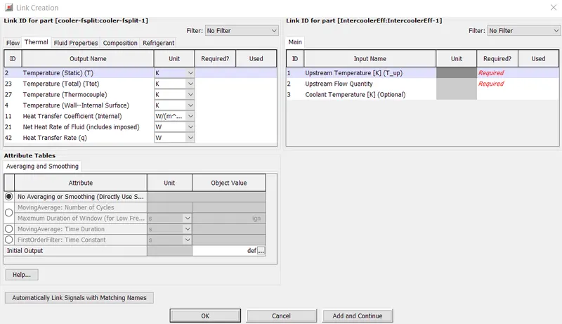
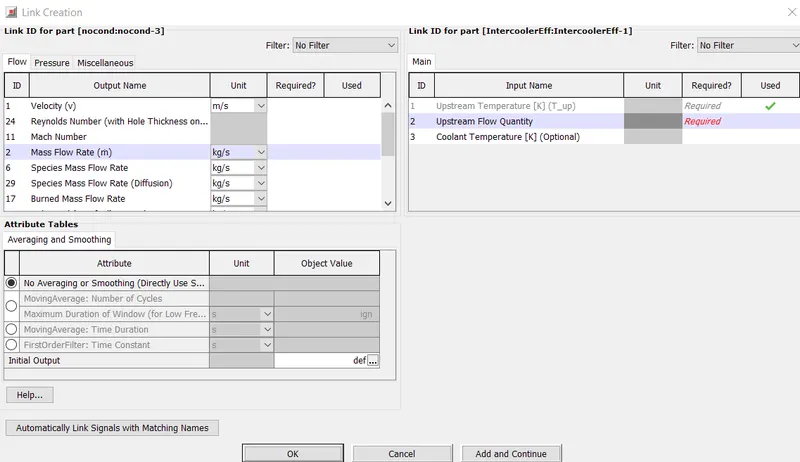
• IntercoolerEff needs the upstream temperature and mass flow as an input to impose a wall temperature on the cooler that will force
  the fluid to exit the cooler at the temperature calculated from the effectiveness table.
• In order to apply intercooler effectiveness, following connections are made;

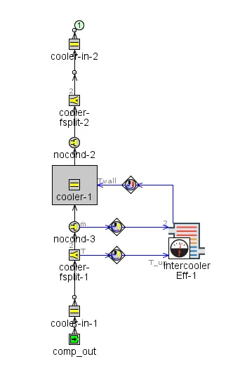
a) Link 1: upstream cooler fsplit is connected to IntercoolerEff in order to sense the upstream temperature.

b)Link 2: inlet orifice is connected to IntercoolerEff in order to share the mass flow rate data.

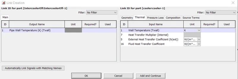
c)Link 3: IntercoolerEff is connected to intercooler to tune the wall temperature as per the effectiveness table data. Coolant Temperature is set to 300K and the below data is assigned.

Intermediate model:

Below is the overview of intercooler model which will be attached to the 6 cylinder DI Engine.

Intake Manifold:

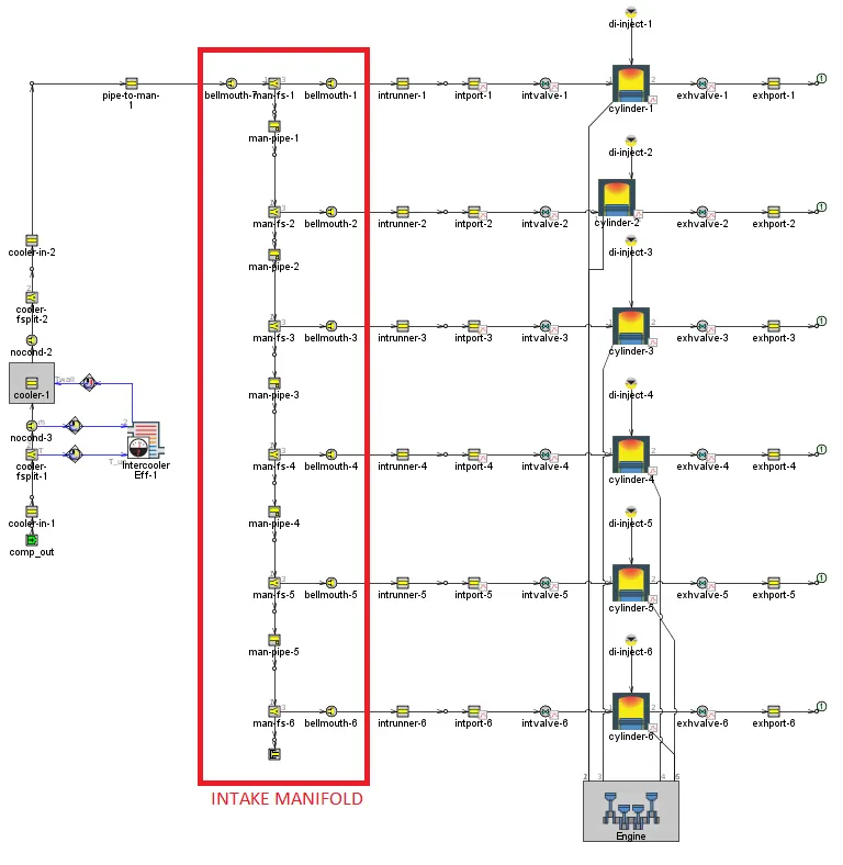
Step 11: Discretization of intake manifold

1. Find your target discretization length. For general performance analysis, the discretization length should be about 0.4 times the bore diameter in the intake system and 0.55 times the bore diameter in the exhaust system. The bore diameter in this model is 100 mm, therefore the intake side discretization length is 40 mm, and the exhaust side discretization length is 55 mm.
2. Determine the location of the flowsplits, ideally allocating one discretization length of length to the flowsplits. Flowsplits are placed first because they always represent 1 sub-volume and cannot be further discretized.
3. Using the overall dimensions, calculate the length remaining for the pipes connecting the flowsplits. Use your intake system target discretization length in the pipes. If any pipes are too short (<0.5*discretization length), their length and volume should be lumped into adjacent flowsplits.

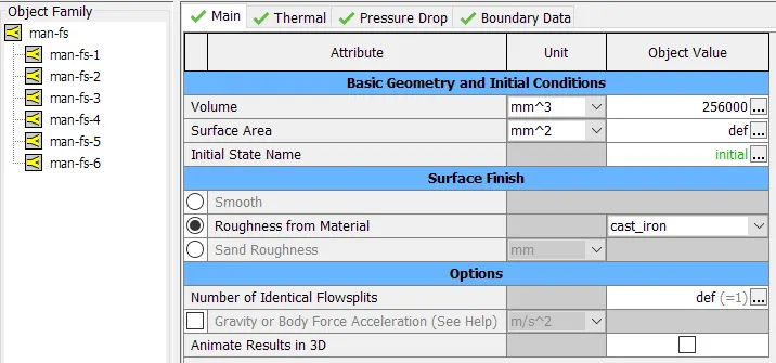
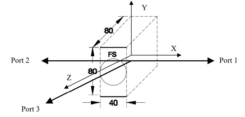
The figure below illustrates the geometry of the flowsplit. The manifold cross section is an 80 by 80 square, so the Volume is 80 mm * 80 mm * 40 mm = 256,000 mm^3. Port 1 is the incoming bulk flow. Port 2 is the outgoing bulk flow. Port 3 is the branch to the intake runner. To determine the attributes for Angle with respect to (wrt) X-axis, Y-axis, and Z-axis choose an arbitrary local coordinate system (there
is no global coordinate system for flowsplits) and draw vectors for each port pointing all out of the flowsplit as shown below. For the local coordinate system shown the Angle wrt X-axis for port 1 is 0°, Angle wrt Y-axis for port 1 is 90°, and Angle wrt Z-axis is also 90°.

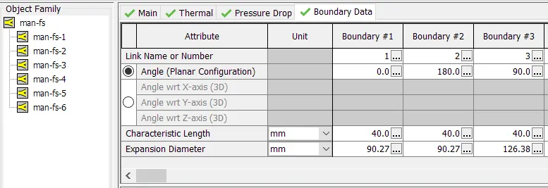
The Expansion Diameter attribute is used to describe the area to which the flow can expand to when entering a port. Flow entering ports 1 and 2 can expand to the diameter equivalent to the 80 by 80 square area, which is diameter 90.27 mm. The expansion diameter of port 3 requires more thought. A value is needed that will indicate to the program how much expansion/contraction loss is associated with the flow
entering/leaving the 90° side branch port 3. The general recommendation for this geometry is an expansion diameter of 1.4 times the bulk flow diameter for a side branch port like port 3. The maximum area that the flow from port 3 could expand to is 2 times the area of port 1. Therefore the maximum expansion diameter for port 3 is square root of 2 times the diameter of port 1, or ~1.4 * 90.27 = 126.38 mm. In reality the expansion diameter depends on both the geometry and the flow characteristics, and could be less than the value specified, but 1.4 times the bulk flow diameter is a good first estimate.

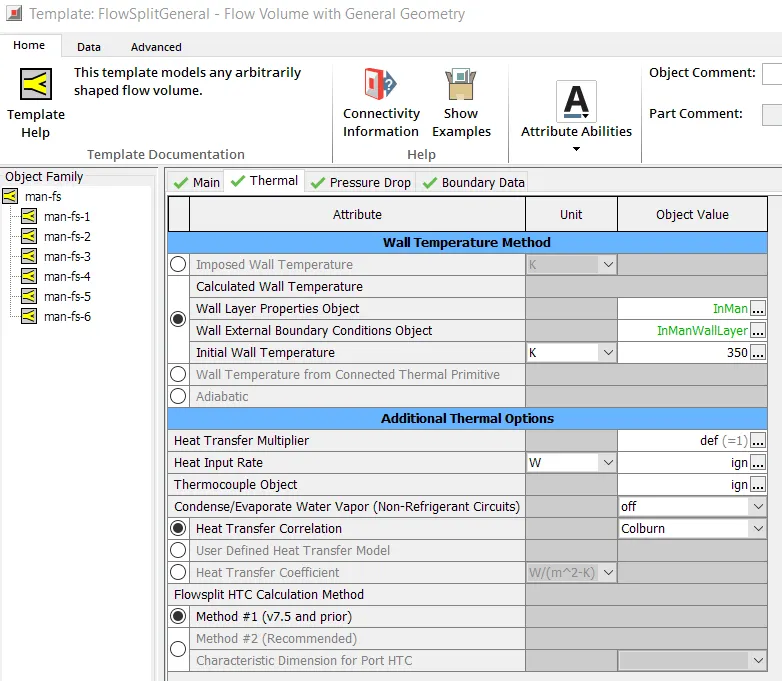
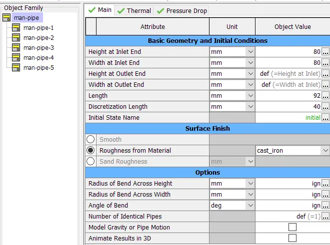
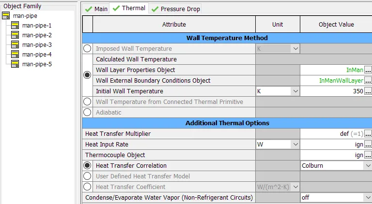
Step 12: Pipe Rectangle element is used to model the square cross section of the manifold. The dimensions are defined as follows with thermal objects as same as applied before for flow splits.

Step 13: The final object needed for the log manifold is an orifice. In most manifolds, the transition from the manifold to the
runners is very smooth. The use of a default orifice in this location would add an additional expansion/contraction loss to the system that is not real. Therefore, the non-default smooth orifice connection called "bellmouth" is needed.

Exhaust Port

The exhaust port must be of 2 outlets as shown below flowing into twin scroll turbine from 3 cylinders each.

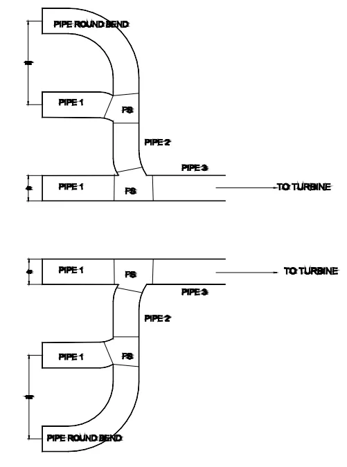
Step 14: Round Pipe with bends and flow splits are used at the exhaust port and the below model of 6cyl DI Engine is obtained without turbocharger.

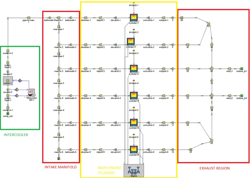
Turbocharging:

Before modelling, it is important to have the following data:
• Measured engine volumetric efficiency or air mass flow data
• Turbine performance map data
• Compressor performance map data
• Measured turbocharger shaft speed data

Step 15: Run the Base Engine Model without the Turbocharger. In this way, the base engine performance can be tested for errors. This would indicate if the base engine model (manifolds, valves, cylinders, etc.) is properly modeled before we start complicating the
system with the turbocharger.

Following data is obtained from the base engine model. In reality, these results has to be checked with the experimental model before introducing turbocharging into the model.

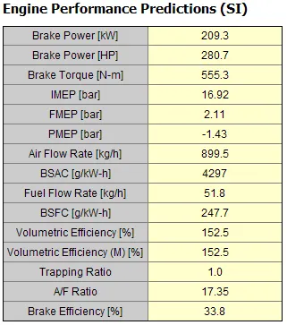
Step 16: Compressor Only Model

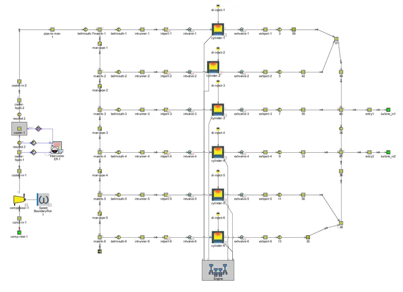
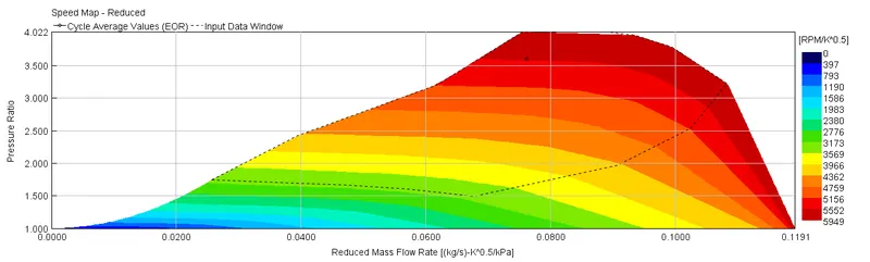
• Compressor is added before the intercooling stage as shown below and a RPM of 96000 is set using the object SpeedBoundaryRot.

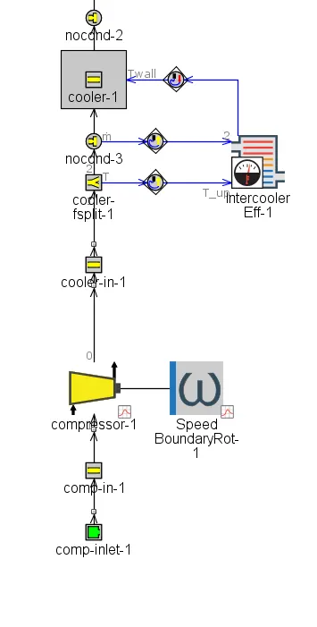
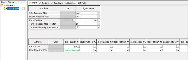
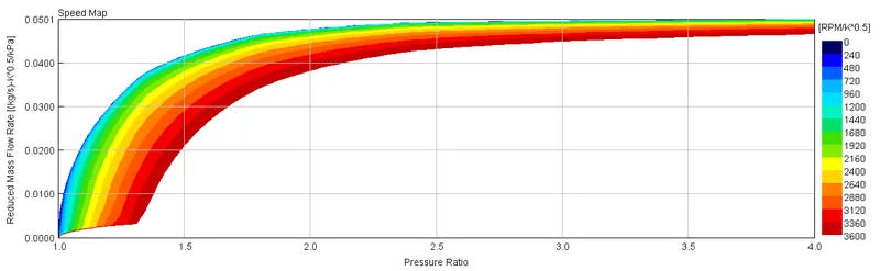
• Compressor inlet is set to 1 bar and 298K. The number of rack position is 1 in the below figure. Rack positions indicate the number of geometrical positions a particular compressor or turbine can be varied. In this case, it is 1. Hence it is a fixed geometry radial compressor.

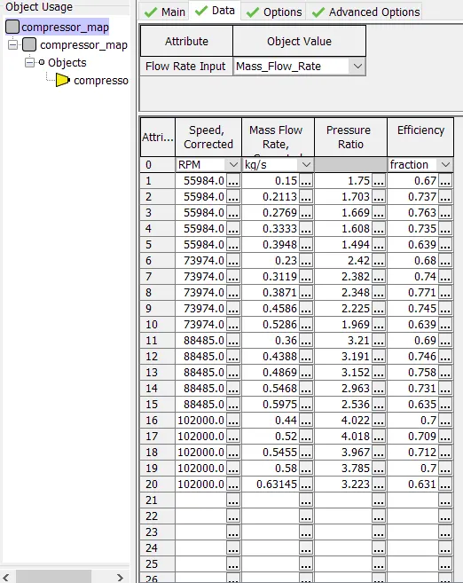
• Compressor Map data is preloaded. It contains data such as the efficienct at particular speeds. Generally this is provided by the supplier to the OEMs.

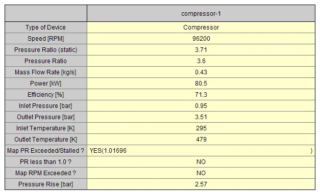
• Result from Compressor Only model and its Operating Map

Step 17: Turbine Only Model

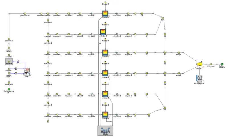
• In this model all the compressor components are removed and replaced using Endenvironment objects. Pressure and Temperature outlet from the Compressor results are noted and applied to the Endenvironment object (Comp out). At the exhaust, turbine is installed.

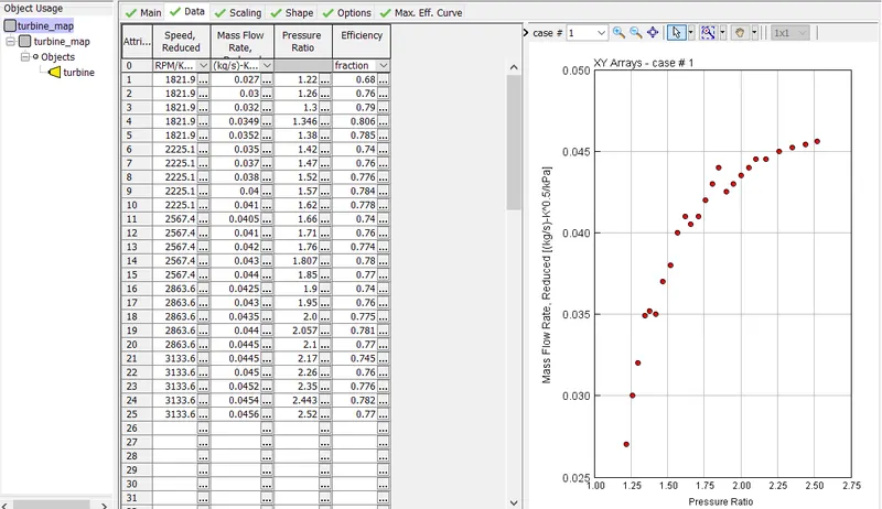
• Similar to Compressor, Turbine also has a map which is provided by the supplier. Various Racks can be added in case of Variable Geometry Turbine.

• Result from Turbine only Model and its Operating Map

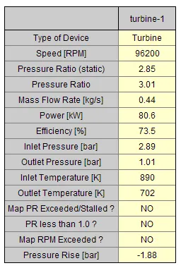
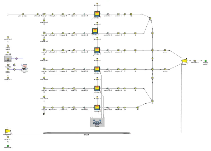
Step 18: The below model is a 6 Cylinder DI Turbocharged Model (Full). It is connected by a common shaft between turbine and compressor. It is evident from the above results that both the Compressor and Turbine produces same amount of Power. This is very much important to validate the model provided all other engine parameters are under satisfactory limits.

PART II-Diesel VGT EGR:

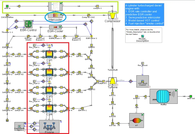
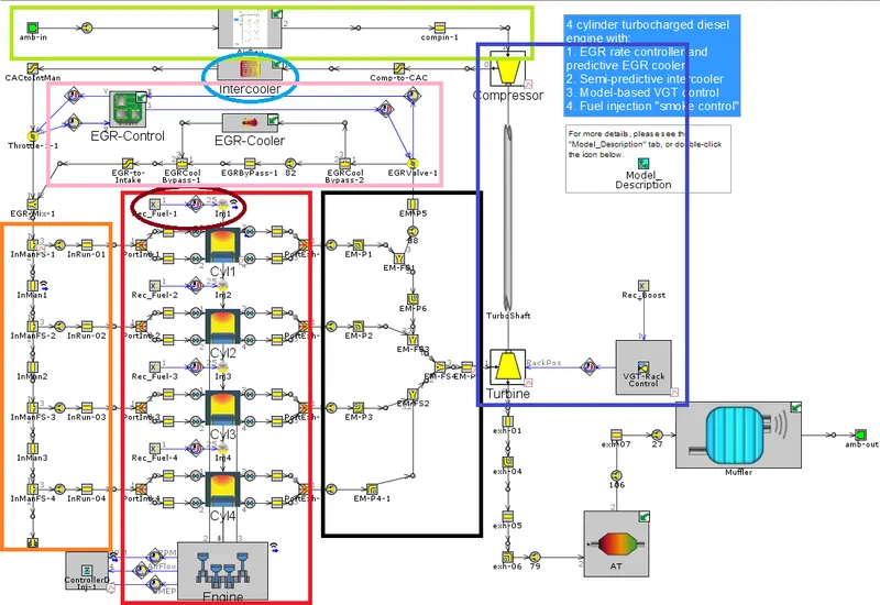
• The example 'Diesel_VGT_EGR' demonstrates several modeling concepts important for automotive diesel engines, including variable geometry turbine, boost control, intercooler, EGR circuit with cooler and EGR rate control, injection limiting for smoke control, and exhaust after treatment device modeling (geometry only, no chemistry).
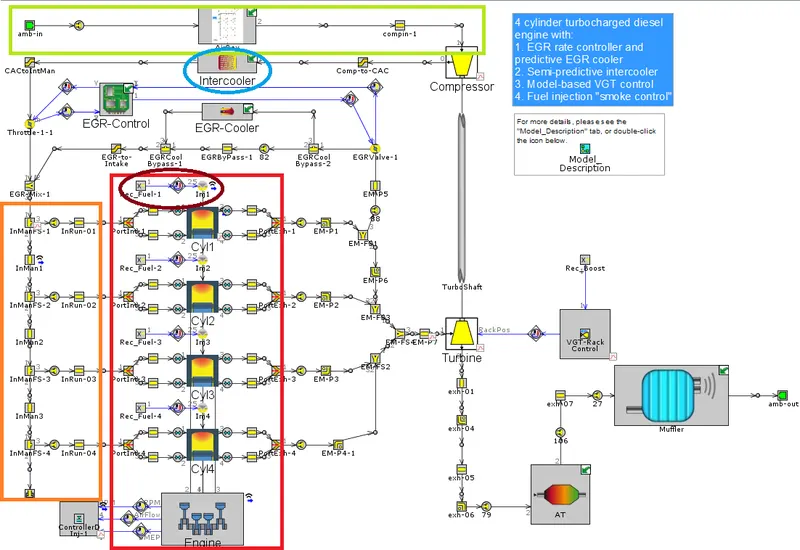
• Engine: The engine is a 4-cylinder, four-stroke, direct injection, 2L diesel engine. The engine runs in "speed" mode, where the engine speed is entered by the user and the engine torque is calculated. Combustion is modeled by the DIPulse method, a predictive combustion model using the detailed injection profiles. In-cylinder heat transfer is modeled using the Woschni model. A FE model is used to predict the cylinder, head and piston temperatures. This simulation will run until it reaches steady-state convergence for six different engine speeds at full load, three part load operating points, and an additional idle point (total of 10 cases).

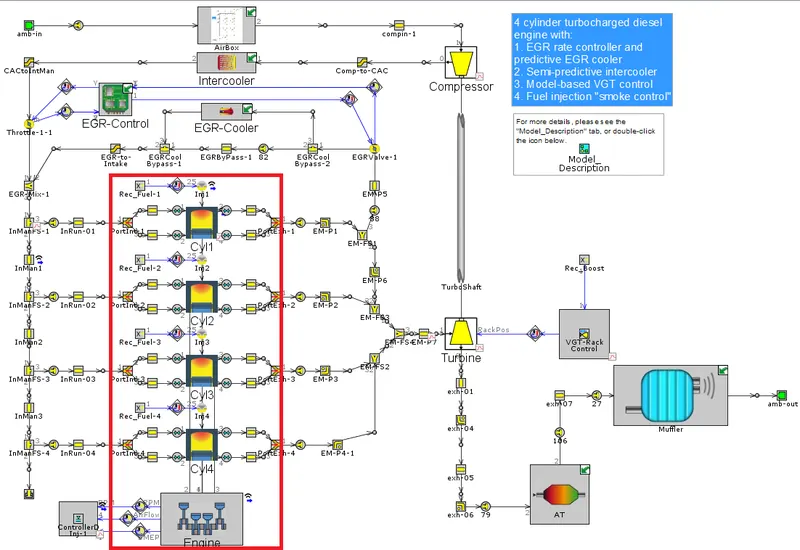
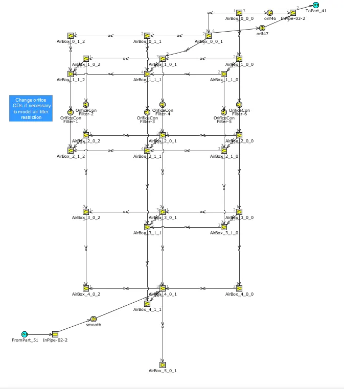
• Intake System: The intake system consists of the air piping upstream of the compressor inlet, and contains a simple model of an air box. The air box is modeled as a group of interconnected flowsplits that represent the total volume of the air box. At the inlet and outlet of the air box, "bellmouth" orifice connections are used to model smooth transitions.

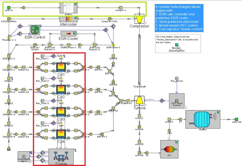
• Below model is a detailed representation of Airbox. It is a discretized model into 1D from a complex 3D geometry.

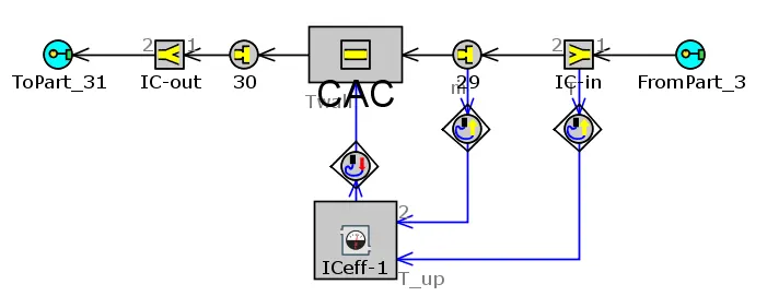
• Intercooler: The intercooler is found downstream of the compressor outlet. This intercooler is an air-to-air intercooler that is modeled using a "semi-predictive" method based on heat exchanger effectiveness. Note that if heat exchanger performance data is available, it is generally preferred to model the heat exchanger using 'HxMaster' and 'HxSlave' parts (which will use the available data to create non-dimensional Nusselt correlations defining heat exchanger performance). This approach will generally extrapolate better than an assumed effectiveness to conditions beyond those present in the heat exchanger data. However, if heat exchanger data is not available (or if the simulation will be run at conditions where HX effectiveness is well known), the semi-predictive effectiveness method is appropriate.
  
  

• The intercooler is modeled using a pipe part. The Number of Identical Pipes attribute is used to model a bundle of 25 identical pipes of 7.0 mm diameter each (giving a large surface area for heat transfer). The pressure drop across the intercooler is calibrated using the Friction Multiplier in the in the pipe. Flowsplits are required to model the inlet and outlet of the intercooler since pipes cannot connect to pipes with the Number of Identical Pipes attribute greater than one. The desired intercooler outlet temperature is calculated by a simple control system and is imposed by actuating the wall temperature of the intercooler pipe. The Heat Transfer Multiplier in the pipe is increased to a large enough value so that the outlet temperature matches the wall temperature. The desired outlet temperature is calculated in a 'IntercoolerEff' part from the effectiveness table of the intercooler.

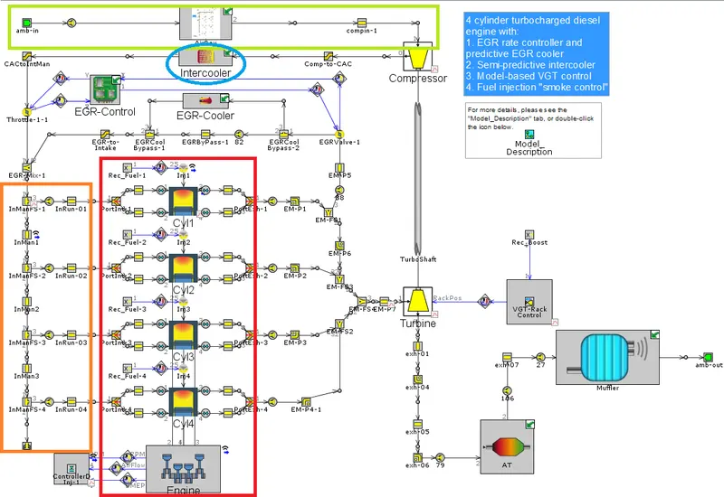
• Intake Manifold: The intake manifold is modeled as aluminum using heat conduction objects to calculate the wall temperatures. This is important in turbocharged models since wall temperatures may change substantially at different operating points, thus influencing the cylinder inlet temperature. The orifices that connect. The initial conditions are different from ambient conditions. The initial temperatures and pressures are specified at the expected boost pressure in order to decrease the convergence time.

• Fuel Injection System: The fuel is injected directly into the cylinders. Both the injection timing and the injection profile are looked up using an 'RLTDependence' as a function of engine speed and injection rate. There is a simple control system that determines the total injected fuel mass (mg/stroke). This control system begins with a 'SignalGenerator' part that imposes an accelerator pedal position input. The "requested fuel mass" is then looked up as a function of engine speed and pedal position. In some cases, the requested fuel mass may produce excess smoke if the boost pressure is not high enough to provide enough air. Therefore, the maximum allowed fuel mass is looked up as a function of the engine speed and the boost pressure. A 'MinMax' part is used to take the smaller of the requested fuel mass and the smoke limited fuel mass. This value is then imposed on the injectors using an actuator.

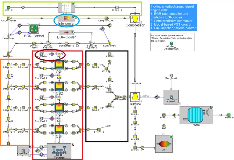
• Exhaust System: The exhaust manifold is modeled as cast iron using heat conduction objects to calculate the wall temperatures. This is very important in the exhaust manifold since wall temperatures change substantially between full load and idle condition, thus influencing the turbine inlet temperatures and turbine power. The orifices that connect the exhaust ports to the runners do not allow heat to be conducted between the pipe walls of the adjacent parts. This is necessary because the wall temperature is calculated in the exhaust pipes, while it has been imposed in the port (the imposed value is artificially high to account for heat transfer from the valve). The initial conditions are different from ambient conditions. The initial temperatures and pressures are specified at the expected backpressure in order to decrease the convergence time. The turbine part references a map file from which map data is read.

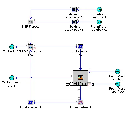
• Exhaust Gas Recirculation: The model includes an exhaust gas recirculation (EGR) system to transport exhaust gases from the exhaust manifold back to the intake manifold. The EGR flow is driven by a positive pressure difference between the exhaust manifold and intake manifold and is controlled by an orifice connection (EGR-valve). The EGR-valve diameter is imposed by an actuator, and is determined automatically by an 'ControllerEGRValve' part to achieve a target EGR fraction. The desired EGR fraction is mapped as a function of engine speed and the requested BMEP. EGR rates in the model are as high as 40% at some operating points. Because of the high EGR rates, it is desirable to cool the EGR gases using a heat exchanger (EGR-cooler). When the pressure drop across the EGR system is not sufficient to achieve the target EGR rate, a throttle in the intake system, controlled by a PID controller, increases the pressure difference. This controller is only active, if the EGR-valve is fully open.

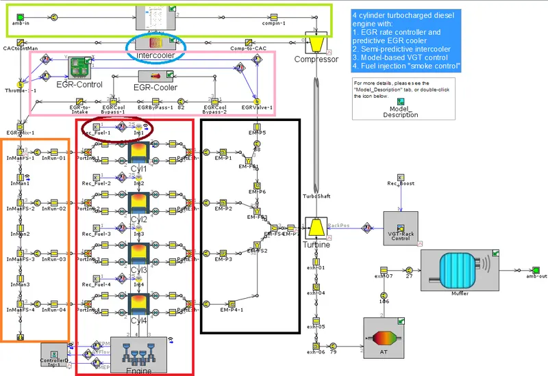
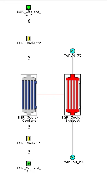
• The EGR cooler is modeled using 'HxMaster' and HxSlave' parts. Coolant side boundary conditions are imposed. The heat exchanger model inputs include geometry along with measured heat transfer and pressure drop performance data. During model pre-processing, the measured data is used to generate non-dimensional correlations for heat transfer that allow the model to accurately predict heat transfer rates at any operating condition. The pressure drop data is use to automatically calibrate physical characteristics (friction multiplier, orifice Cd) of the heat exchanger so that the data is well matched.

• Turbocharger: The turbocharger in this model contains a fixed geometry compressor and a variable geometry turbine (VGT). For the VGT, there are 5 different sets of turbine map data entered at each of 5 VGT rack positions. The VGT rack position is determined by a control system to achieve a target boost pressure upstream of the intake manifold. The boost pressure is sensed and is then filtered using a 'MovingAverage' part to produce an average pressure signal. The model based controller compares the sensed boost pressure to the target boost pressure and then adjusts the VGT rack position accordingly.

• Exhaust System: A full vehicle exhaust system is modeled downstream of the turbine outlet. The geometry of a Diesel Oxidation Catalyst (DOC) is modeled using a 'CatalystBrick' part. In this example only the pressure drop across the DOC is of interest, so no chemical reactions are modeled in the DOC. The inlet and outlet of the DOC must be modeled using flowsplits because the DOC is effectively a bundle of very small pipes.

  Just downstream of the DOC is a Diesel Particulate Filter (DPF) using a 'DieselParticFilter' part. In this example, only the geometry attributes are specified so that proper pressure drop across the filter is modeled, but there is no soot accumulation or regeneration modeled. Similar to the DOC, the inlet and outlet of the DPF must be modeled using flowsplits.

  Downstream of the DOC is a muffler. This muffler was modeled using GEM3D, which enables complex muffler geometry to be entered in a CAD tool and automatically discretized into a GT-POWER model. The muffler in this example is a tri-flow type muffler with two baffles. The center chamber between the two baffles is filled with wool, and various internal pipes and baffles include perforation. The .gem file is included in the directory and can be opened in GEM3D to see the muffler. The output of the GEM discretization is stored within an internal subassembly to keep the main project map clean.

  
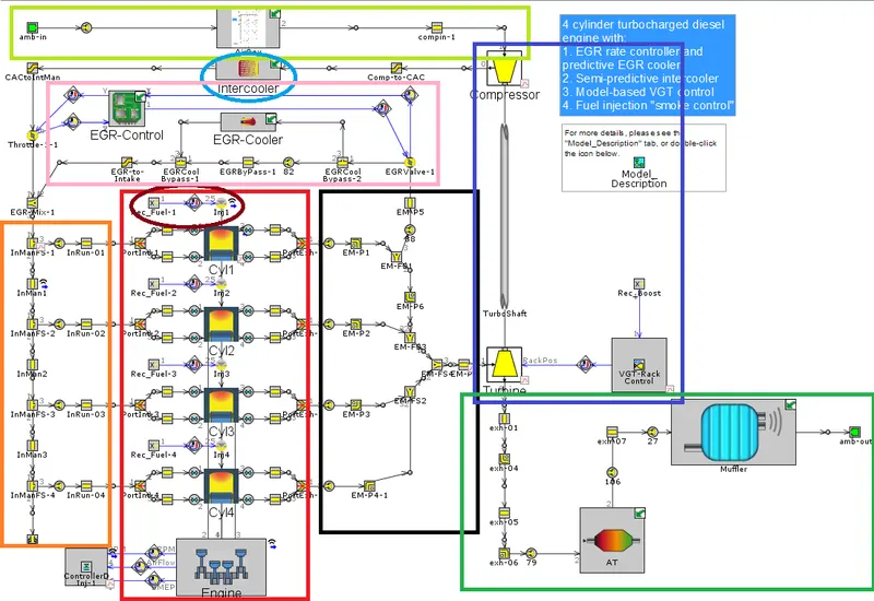
• DOC and DPF Aftertreatment devices are the first stage of aftertreatment devices located inside "AT
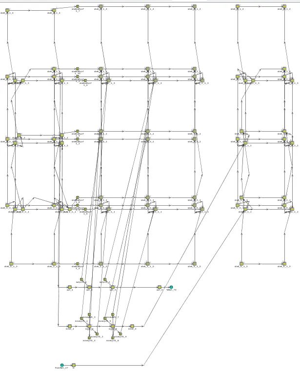
• Downstream of the DOC is a muffler. This muffler was modeled using GEM3D, which enables complex muffler geometry to be entered in a CAD tool and automatically discretized into a GT-POWER model. The muffler in this example is a tri-flow type muffler with two baffles. The center chamber between the two baffles is filled with wool, and various internal pipes and baffles include perforation. The .gem file is included in the directory and can be opened in GEM3D to see the muffler. The output of the GEM discretization is stored within an internal subassembly to keep the main project map clean. Muffler Geometry is discretized to 1D model from 3D using GEM3D and the resultant model is as below.

References:

[1] Internal Combustion Engines Fundamentals, John B Heywood

[2] https://www.melett.com/technical/turbocharger-explained/types-of-turbocharger/