Week 6 - Multivariate Newton Rhapson Solver

Week 6 - Multivariate Newton Rhapson Solver

Aim:- To solve the a given set of 'ODE system of coupled non-linear equations', by using the Multivariate Newton Rhapson Solver.

Introduction:- The Multivariate Newton -Rhapson Method is a direct extension of the single variable Newton-Raphson Method.

Where the single variable Newton Rhapson Method solved,

f(x) =0, the multivariate version will solve a system of n equations of the form:

`f_1 =(x_1,x_2,x_3,.....) =0`

`f_2 =(x_1,x_2,x_3,.....) =0`

`f_3 =(x_1,x_2,x_3,.....) =0`

'

'

'

`f_(n-1) =(x_1,x_2,x_3,.....) =0`

`f_n =(x_1,x_2,x_3,.....) =0`

we will adopt the shorthand notation for the equation

f(x) =0

According to 'Multivariate Newton Rhapson Method', to get the solution out of coupled non-linear ODE below equation we use:

`y_n =y _(old) - alpha * J^-1 *F`

where, alpha -relaxation factor

Vector F will be written as,

`f=((f_1),(f_2),(f_3))`

old value or guess value will be written as,

`y _(old)=((y_1old),(y_2old),(y_3old))`

Jacobian Matrix,

`J=[[(df_1)/dy_1,(df_1)/dy_2,(df_1)/dy_3],[(df_2)/dy_1,(df_2)/dy_2,(df_2)/dy_3],[(df_3)/dy_1,(df_3)/dy_2,(df_3)/dy_3]]`

where, number of column = number of independent variables

number of rows = number of Functions

Code:-

"""
# Implicit Euler Method/Backward Differencing Scheme
Program to solve the ODE system of coupled non-linear  equations
	dy1/dt=(-0.04*y1)+(10^44*y2*y3)
	dy2/dt =(0.04*y1 -(10^4*y2*y3) -(3*10^7*y2^2)
	dy3/dt = (3*10^7*y2^2)
"""
#libraries
import matplotlib.pyplot as plt  # plotting the graph
import numpy as np   # matrix manipulation, calculations
from numpy.linalg import inv  # 'linalg (linear algebra)' package from the 'numpy',inv (inverse) for 'Jacobian Inverse'



# First non-linear equation
def f1(y1,y2,y3,y1_old,dt):
	return y1_old + dt*(-0.04*y1 + (pow(10,4)*y2*y3)) - y1
# Second non-linear equation
def f2(y1,y2,y3,y2_old,dt):
	 
	return y2_old + dt*(0.04*y1 - (pow(10,4)*y2*y3) - (3*pow(10,7)*pow(y2,2))) - y2
 #Third non-linear equation
def f3(y1,y2,y3,y3_old,dt):
	
    return y3_old + dt*(3*pow(10,7)*pow(y2,2)) - y3

#Define the Jocobian Matrix
def jacobian(y1,y2,y3,y1_old,y2_old,y3_old,dt):
	
	J = np.ones((3,3))
	
	dy=1e-4
	#Row 1
	J[0,0] =  (f1(y1+dy,y2,y3,y1_old,dt) - f1(y1,y2,y3,y1_old,dt))/dy
	J[0,1] =  (f1(y1,y2+dy,y3,y1_old,dt) - f1(y1,y2,y3,y1_old,dt))/dy   
	J[0,2] =  (f1(y1,y2,y3+dy,y1_old,dt) - f1(y1,y2,y3,y1_old,dt))/dy 

	#Row 2
	J[1,0] = (f2(y1+dy,y2,y3,y2_old,dt) - f2(y1,y2,y3,y2_old,dt))/dy
	J[1,1] = (f2(y1,y2+dy,y3,y2_old,dt) - f2(y1,y2,y3,y2_old,dt))/dy
	J[1,2] = (f2(y1,y2,y3+dy,y2_old,dt) - f2(y1,y2,y3,y2_old,dt))/dy

	#Row 3
	J[2,0] = (f3(y1+dy,y2,y3,y3_old,dt) - f3(y1,y2,y3,y3_old,dt))/dy
	J[2,1] = (f3(y1,y2+dy,y3,y3_old,dt) - f3(y1,y2,y3,y3_old,dt))/dy
	J[2,2] = (f3(y1,y2,y3+dy,y3_old,dt) - f3(y1,y2,y3,y3_old,dt))/dy

	return(J)

#  given 'initial guess values' 
# numpy column vecotr
y_old = np.zeros((3,1))
y_old[0] = 1   # decalring the conditions provided for the y1
 
F =np.zeros((3,1)) # you can declare the F vector as zeros as they are going to change with the iterations 
y_new = np.zeros((3,1))  # variable used to update the Y's in the while loop for every time step 
dy = 1e-4  # differential parameters

# parameters for newton rhapson solver
alpha =1   # relaxation factor 'given '
T = 60 # 600sec
dt = 0.1  # step size

n =int(T/dt) # no.of grid points
print(n)      # print the 'grid points'
time =np.arange(0,n)  # time  between '0' to 'n' 
print(time)          # print the 'time'
 
y_new1 =[]   # new values of 'y1' stored in the array
y_new2 =[]   # new values of 'y2' stored in the array
y_new3 =[]   # new values of 'y3' stored in the array

# starting the newton rhapson loop
iter =1  # initial the of 'iteration values'

for i in range(0,len(time)):
	error =9e9    # assume the error value
	tol = 1e-6    # assume tolerance value
	y_guess = np.copy(y_old)  ## Running while loop with the guessed values of 'y' untill the Final value is obtained for that time step
	print(i)      
	while error >tol:
	# computing the Jacobian -old values are used
		J = jacobian(y_new[0],y_new[1],y_new[2],y_old[0],y_old[1],y_old[2],dt)

		F[0]=f1(y_guess[0],y_guess[1],y_guess[2],y_old[0],dt)
		F[1]=f2(y_guess[0],y_guess[1],y_guess[2],y_old[1],dt)
		F[2]=f3(y_guess[0],y_guess[1],y_guess[2],y_old[2],dt)

	# computing new values
		y_new= y_guess - alpha*np.matmul(inv(J),F)  ## We are updating the y_guess over the while loop until the error becomes less than tolerance
		error=max(abs(y_new-y_guess))  # error values
		y_guess= y_new         # you need to update the guess vector until the while loop is satisfied
	

	#updating the old values 
	y_old = y_new
	y_new1.append(y_new[0])
	y_new2.append(y_new[1])
	y_new3.append(y_new[2])
		
 
#plotting
plt.plot(time,y_new1,color='red',label='y new1')
plt.plot(time,y_new2,color='blue',label='y new2')
plt.plot(time,y_new3,color='green',label='y new3')
plt.xlabel('Simulation Time in s')
plt.ylabel('y new values')
plt.title('Simulation Time versus y new values')
plt.grid('on')
plt.legend(fontsize = 10)
plt.show()

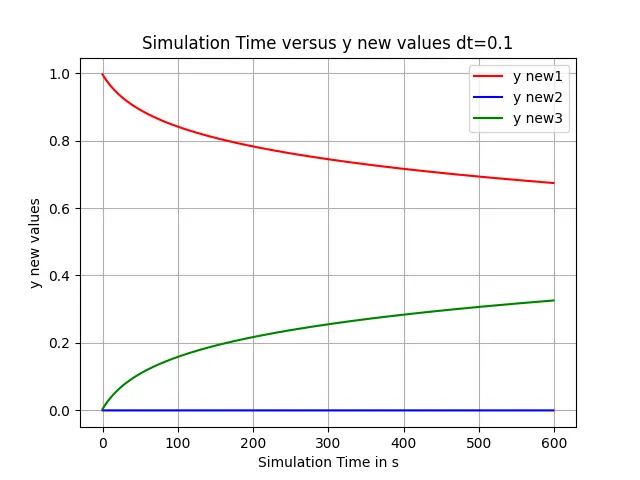
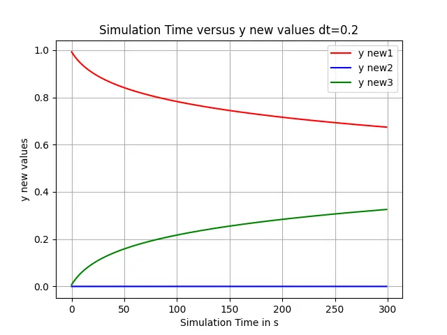
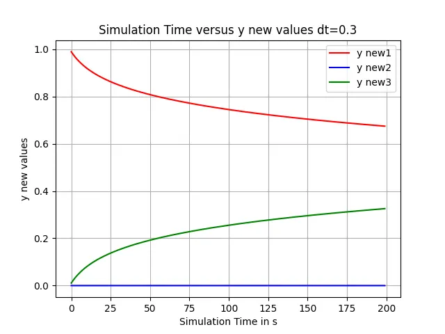
Conclusion:- In the above graphs, the simulation time run at 10 mintues @ ideal step size (dt=0.1). while , changing the 'dt =0.2 @ simulation time (300 s) & dt =0.3 @ simulation time (200 s).' Therefore, increase the time step size (dt) reduces the 'simulation time'.

********************