Week 6 - Multivariate Newton Rhapson Solver

Aim:

To solve the system of equations using multivariate newton raphson solver.

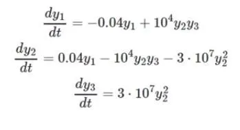
From the equations above they are coupled and can only be solved by the set of equations. These types of equations are generally stiff and are solved with implicit technique. Here for each time phase newton raphson is used. As for each time frame there are more than one unknown multivariate newton approximation is used. The general formula for multivariate newton approximation can be seen below:

`underset(n+1)(X) = underset(n)(X) - alpha.J^(-1).F`

The matrix representation can be seen below

`underset(n+1)([[underset(1)(x)],[.],[.],[.],[underset(n)(x)]]) = underset(n)([[underset(1)(x)],[.],[.],[.],[underset(n)(x)]]) - [J^(-1).underset(n)(X)][[underset(1)(f(x))],[.],[.],[.],[underset(n)(f(x))]]`

Alpha is multiplied in the above figure to the jacobian reverse and the word matrix and the function. Jacobian matrix is calculated numerically as analytical derivates are always not present. The numerical jacobian can be calculated as follows:

`frac{dunderset(i)(f)}{dunderset(j)(x)} = frac{f(underset(j)(x) + h) - f(underset(j)(x))}{h}`

We also use implicit method for the outer integration loop for this task. The backward differencing method is thus used and the general method is shown below:

`f'(x) = frac{f(x) - f(x-h)}{h}`

The initial conditions are provided in the problem statement and are shown below:

`underset(1)(y) = 1`

`underset(2)(y) = 0`

`underset(3)(y) = 0`

Here we are initializing the ODE's in the form:

`f'(x) = underset(old value)(x) + dt.f(x) - underset(n ew value)(x)`

The general layout of the code can be seen below:

• ODE time integration loop
• Assembling ODE system
• Newton raphson solver until convergence
• Get the updated values
• End of outer loop

The code can be seen below:

'''
program to solve coupled differential equations using multivariate newton raphson technique
dy1/dt = -0.04y1 + 10^4 y2*y3
dy2/dt = 0.04y1 - 10^4 y2*y3 - 3*10^7*y2^2
dy3/dt = 3*10^7 y2^2
The bde for implicit function becomes 
f(x_i) = hf'(x_i) + f'(x_i-1)
Thus the function becomes
f1 = y1^(i-1) + h(-0.04y1 + 10y2y3) - y1^i
f2 = y2^(i-1) + h(0.04y1 - 10^4y2y3 - 3e7y2^2) - y2^i
f3 = y3^(i-1) + h(3e7y2^2) - y3^i
'''
import numpy as np
from numpy.linalg import inv
import matplotlib.pyplot as plt

t_initial = 0
t_final = 600
dt = 50

#initial guess values
y1 = 1
y2 = 0
y3 = 0

def f1(y1_old,y1,y2,y3,dt):
	return y1_old + dt*(-0.04*y1 + pow(10,4)*y2*y3) - y1

def f2(y2_old,y1,y2,y3,dt):
	return y2_old + dt*(0.04*y1 - pow(10,4)*y2*y3 - 3*pow(10,7)*pow(y2,2)) - y2

def f3(y3_old,y1,y2,y3,dt):
	return y3_old + dt*(3*pow(10,7)*pow(y2,2)) - y3

def jac(y1_old,y2_old,y3_old,y1,y2,y3,dt):

	j = np.ones((3,3))
	d = 1e-8

	#row1
	j[0,0] = (f1(y1_old,y1+d,y2,y3,dt) - f1(y1_old,y1,y2,y3,dt))/d
	j[0,1] = (f1(y1_old,y1,y2+d,y3,dt) - f1(y1_old,y1,y2,y3,dt))/d
	j[0,2] = (f1(y1_old,y1,y2,y3+d,dt) - f1(y1_old,y1,y2,y3,dt))/d

	#row2
	j[1,0] = (f2(y2_old,y1+d,y2,y3,dt) - f2(y2_old,y1,y2,y3,dt))/d
	j[1,1] = (f2(y2_old,y1,y2+d,y3,dt) - f2(y2_old,y1,y2,y3,dt))/d
	j[1,2] = (f2(y2_old,y1,y2,y3+d,dt) - f2(y2_old,y1,y2,y3,dt))/d
	
	#row1
	j[2,0] = (f3(y3_old,y1+d,y2,y3,dt) - f3(y3_old,y1,y2,y3,dt))/d
	j[2,1] = (f3(y3_old,y1,y2+d,y3,dt) - f3(y3_old,y1,y2,y3,dt))/d
	j[2,2] = (f3(y3_old,y1,y2,y3+d,dt) - f3(y3_old,y1,y2,y3,dt))/d

	return j

y_new = np.ones((3,1))
y_old = np.ones((3,1))
y_guess = np.ones((3,1))

t = np.arange(t_initial,t_final,dt)
total_iter = len(t)
y=np.ones((3,total_iter))

f = np.copy(y_guess)

time_iter = 0
iter = 0
print(y)
print(total_iter)

for i in range(0,total_iter):

	y_old[0] = y1
	y_old[1] = y2
	y_old[2] = y3

	y_guess[0] = y1
	y_guess[1] = y2
	y_guess[2] = y3

	alpha = 1
	tol = 1e-8
	error = 9e9


	while error>tol:
		f[0] = f1(y_old[0],y_guess[0],y_guess[1],y_guess[2],dt)
		f[1] = f2(y_old[1],y_guess[0],y_guess[1],y_guess[2],dt)
		f[2] = f3(y_old[2],y_guess[0],y_guess[1],y_guess[2],dt)

		j = jac(y_old[0],y_old[1],y_old[2],y_guess[0],y_guess[1],y_guess[2],dt)

		y_new = y_guess - alpha*np.matmul(inv(j),f)
		error = np.max(np.abs(y_guess - y_new))

		y_guess = y_new
		log_message = 'iteration # = {0} y1 = {1} y2 = {2} y3 = {3}'.format(iter,y_new[0],y_new[1],y_new[2])
		print(log_message)
		iter = iter + 1

	y1 = y_new[0]
	y2 = y_new[1]
	y3 = y_new[2]

	y[0,time_iter] = y_new[0]
	y[1,time_iter] = y_new[1]
	y[2,time_iter] = y_new[2]

	time_iter = time_iter + 1

plt.plot(t,y[0])
plt.plot(t,y[1])
plt.plot(t,y[2])
plt.legend(['y1','y2','y3'])
plt.grid('on')
plt.xlabel('Simulation Time')
plt.ylabel('initial guess values')
plt.show()

Results:

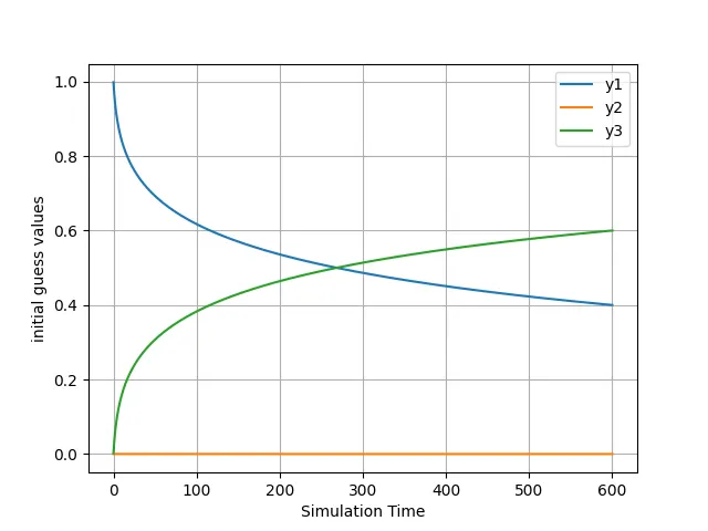
For the time step size of 0.05

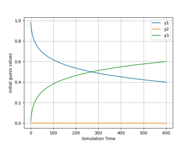
For the time step size of 0.5

For the time step size of 50

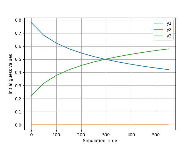
Discussion:

As the solution marches forward in time the values change rapidly, this indicates the stiff behaviour of the system. It can be seen that for all time step size the code gives us the result without any instability. But it can be noticed that results become inconsistent with higher time step size. The unconditional stability can be here seen as reason for the implicit scheme whereas for explicit scheme the time step size would have been too low or else leading to instability.