Week 6 - Multivariate Newton Rhapson Solver

AIM:-

• To solve the below set of equations.

• To Incorporate numerical jacobian.
• To solve the problem using Implicit Euler Method/Backward Differencing.
• To choose a time step and explain what is the ideal step size in this case?

Code and Explanation:-

We are calling this as a Multivariate Newton Raphson because we were solving three species y1, y2 & y3.

Multi Newton Raphson:-

We can see that the above 3 equations are non-linear coupled equations. We can say that these equations are non-linear because of the unknown elements which are going to solve multiply themselves.

Here the Newton Raphson solver is implemented to solve the Non-linear system of coupled equations at each time step using an implicit method.

`Yunderset(n+1)`=`Yunderset(n)`-`alpha*[j^(-1)*f]`

Yn+1 is New values

Yn is Old values

j-1 is Jocabian Matrix is differenciation of the net rate of reaction of each unknown value.

f is function of each equation

Here, the jacobian matrix contains the differentiation of the net rate of reaction of eacch unknown value.

`((Y1n+1),(Y2n+1),(.),(.),(Yn(n+1))) = ((Y1),(Y2),(.),(.))-alpha*[[[dy1/dt],[dy2/dt],[dy3/dt]],[[dy1/dt],[dy2/dt],[dy3/dt]],[[dy1/dt],[dy2/dt],[dy3/dt]]]*((f1),(f2),(f3))`

Code:-

'''
Multinewton raphson method using Implicit Backward

dy1/dt=-0.04y1 + 10^4*y2*y3
dy2/dt= 0.04y1-10^4y2*y3-3*10^7*y2^2
DY3/DT=3*10^7

Using Implicit Backward Difference Method

x_new= x_old-(f(x))*dt

f1=y1_old-(0.04*y1-10^4*y1*y3)*dt-y1_new
f2=y2_old+(0.04*y4-10^4*y2*y3-3*10^7*y2^2)*dt-y2_new
f3=y3_old+(3*10^7*y2^2)*dt-y3_new

'''
import math
import numpy as np
from numpy.linalg import inv
import matplotlib.pyplot as plt

def f1(y1_old,y1,y2,y3,dt):
	return y1_old+dt*(-0.04*y1+pow(10,4)*y2*y3)-y1

def f2(y2_old,y1,y2,y3,dt):
	return y2_old+dt*(0.04*y1-pow(10,4)*y2*y3-3*pow(10,7)*pow(y2,2))-y2

def f3(y3_old,y1,y2,y3,dt):
	return y3_old+dt*(3*pow(10,7)*pow(y2,2))-y3

def jacobian(y1_old,y2_old,y3_old,y1,y2,y3,dt):

	J=np.ones((3,3))
	d=1e-8
	#Derivative of each function
	J[0,0]=(f1(y1_old,y1+d,y2,y3,dt)-f1(y1_old,y1,y2,y3,dt))/d
	J[0,1]=(f1(y1_old,y1,y2+d,y3,dt)-f1(y1_old,y1,y2,y3,dt))/d
	J[0,2]=(f1(y1_old,y1,y2,y3+d,dt)-f1(y1_old,y1,y2,y3,dt))/d

	#Derivative of second function
	J[1,0]=(f2(y2_old,y1+d,y2,y3,dt)-f2(y2_old,y1,y2,y3,dt))/d
	J[1,1]=(f2(y2_old,y1,y2+d,y3,dt)-f2(y2_old,y1,y2,y3,dt))/d
	J[1,2]=(f2(y2_old,y1,y2,y3+d,dt)-f2(y2_old,y1,y2,y3,dt))/d

	#Derivative of third function
	J[2,0]=(f3(y2_old,y1+d,y2,y3,dt)-f3(y2_old,y1,y2,y3,dt))/d
	J[2,1]=(f3(y2_old,y1,y2+d,y3,dt)-f3(y2_old,y1,y2,y3,dt))/d
	J[2,2]=(f3(y2_old,y1,y2,y3+d,dt)-f3(y2_old,y1,y2,y3,dt))/d

	return J 

#Initial Values
y1=1
y2=0 
y3=0

#Time loop
t_start=0
t_end=600
dt=0.1
t=np.arange(t_start,t_end)
time=len(t)

#Final values
y1_new=[]
y2_new=[]
y3_new=[]

for i in range(1,time+1):

	error = 9e9
	tol=1e-6
	alpha=1  

	y_old=np.ones((3,1))

	y_old[0]=y1
	y_old[1]=y2
	y_old[2]=y3 

	#Guess values
	y_guess=np.ones((3,1))
	y_guess[0]=y1 
	y_guess[1]=y2 
	y_guess[2]=y3 

	f=np.ones((3,1))
	iter=0

	while error>tol:

		#Jocobian using Numerical Method

		J=jacobian(y_old[0],y_old[1],y_old[2],y_guess[0],y_guess[1],y_guess[2],dt)

		f[0]=f1(y_old[0],y_guess[0],y_guess[1],y_guess[2],dt)
		f[1]=f2(y_old[1],y_guess[0],y_guess[1],y_guess[2],dt)
		f[2]=f3(y_old[2],y_guess[0],y_guess[1],y_guess[2],dt)

		y_new=y_guess - alpha*np.matmul(inv(J),f)
		error=np.max(np.abs(y_new-y_guess))


		#update y_guess
		y_guess=y_new
		value=('iter #={0} x1={1} x2={2} x3={3}'.format(iter,y_new[0],y_new[1],y_new[2]))

		#print(value)

		iter=iter+1

	y1=y_new[0]
	y2=y_new[1]
	y3=y_new[2]


	y1_new.append(y_new[0])
	y2_new.append(y_new[1])
	y3_new.append(y_new[2])
	

# Plot

plt.plot(t,y1_new)
plt.plot(t,y2_new)
plt.plot(t,y3_new)
plt.xlabel('Simulation Time(sec)')
plt.title('Multiraphson method dt=0.1')
plt.legend(['y1','y2','y3'])
plt.show()

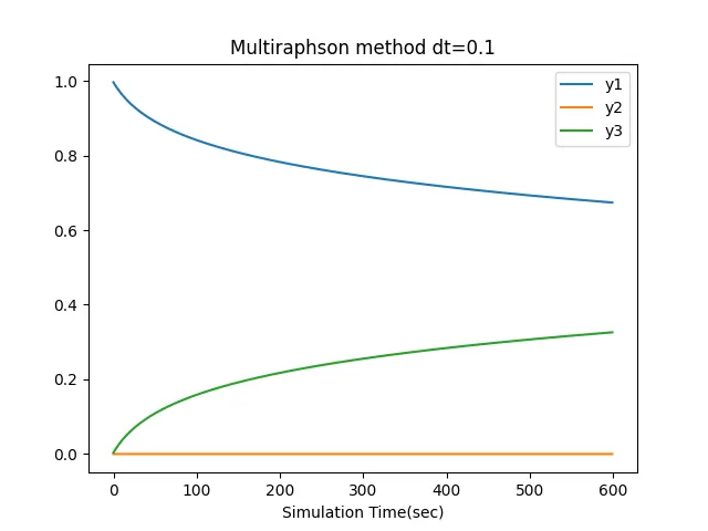
For dt=0.1 and alpha=1

the plot is

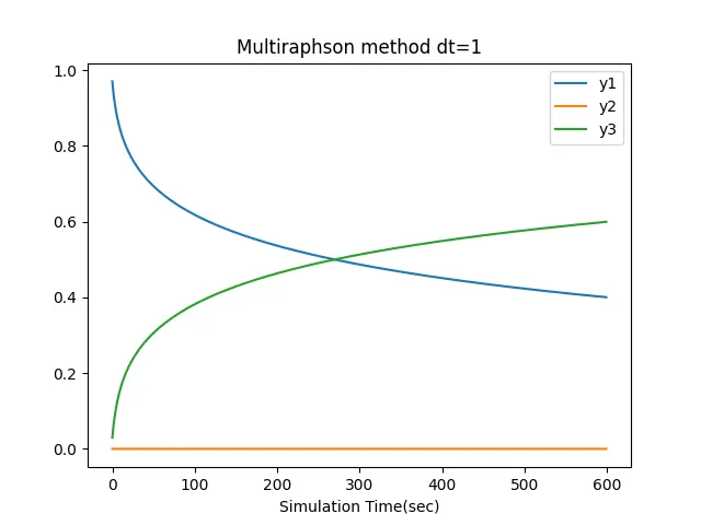
For Dt=1and alpha=1

the plot is

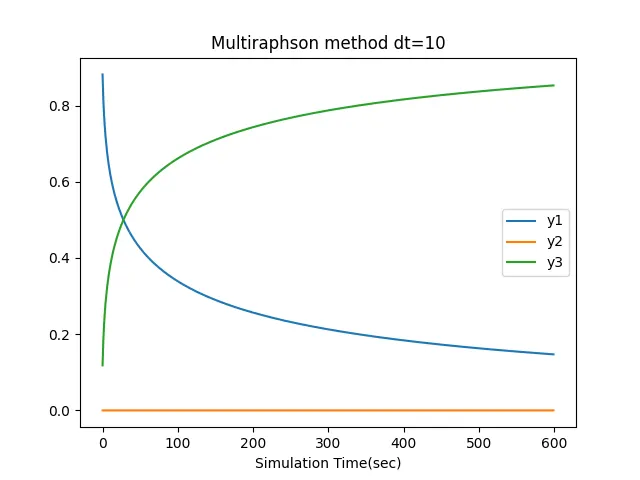
For dt=10 and apha=1

Conclusion:-

We have executed the code for 10 mins. So with the above plot outputs we can see different plots for varying the dt values.

As we increase the dt values the solution is not getting stable and the initial values are moving out.

Plots dt<0.1 is giving stable output. So we can say that the value less than 0.1 is ideal case for this problem.