Week 6 - Multivariate Newton Rhapson Solver

Newton Raphson Method:

The generalized version of multivariate newton raphson method can be expressed as:

`Y_{"new"} = Y_{"guess"} - alpha*(J^{-1}*F)`

Where,

J is the jacobian matrix

F is the algebriac function

Y is the solution vector

The given Differential Equation:

`{dy_1}/{dt} = -0.04y_1 + 10^4y_2y_3`

`{dy_2}/{dt} = 0.04y_1 + 10^4y_2y_3 -3*10^7*y_2^2`

`{dy_3}/{dt} = 3*10^7*y_2^2`

Applying the backward difference method:

`{y_1^n - y_1^{n-1}}/{Deltat} = -0.04y_1^n + 10^4*y_2^n*y_3^n`

Similarly,

`{y_2^{n} - y_2^{n-1} }/{dt}= 0.04y_1^n - 10^4y_2^n*y_3^n - 3*10^7(y_2^n)^2`

Similarly,

`{y_3^n - y_3^{n-1}}/{dt} = 3*10^7*(y_2^n)^2`

Where,

`f_{1,2,3}^{n}` is the function at current time step

`f_{1,2,3}^{n-1}` is the function at previous time step

The algebriac functions to be used in newton raphson method:

`f_1^n = y_1^n + Deltat(0.04y_1^n - 10^4y_2^ny_3^n) - y_1^(n-1) = 0`

`f_2^n = y_2^n - Deltat(0.04y_1^n - 10^4y_2^ny_3^n -3*10^7(y_2^n)^2) - y_2^(n-1) = 0`

`f_3^n = y_3^n - Delta(3*10^7(y_2^n)^2) - y_3^(n-1) = 0`

`J = [[{delf_1^{n}}/{dely_1^{n}}, {delf_1^{n}}/{dely_2^{n}}, {delf_1^{n}}/{dely_3^{n}}],[{delf_2^{n}}/{dely_1^{n}}, {delf_2^{n}}/{dely_2^{n}}, {delf_2^{n}}/{dely_3^{n}}],[{delf_3^{n}}/{dely_1^{n}}, {delf_3^{n}}/{dely_2^{n}}, {delf_3^{n}}/{dely_3^{n}}]]`

The Solution code:

import numpy as np 
import matplotlib.pyplot as plt
from numpy.linalg import inv

# Functions definition as described above
def f1(y1,y2,y3,y_old1,dt): 
	return y_old1 + dt*(-0.04*y1 + (pow(10,4)*y2*y3)) - y1

def f2(y1,y2,y3,y_old2,dt): 
	return y_old2 + dt*(0.04*y1 - (pow(10,4)*y2*y3) - (3*pow(10,7)*pow(y2,2))) - y2

def f3(y1,y2,y3,y_old3,dt): 
	return y_old3 + dt*(3*pow(10,7)*pow(y2,2)) - y3

# Jacobian matrix definition
def jacobian(y_new,y_old,dt):

	# Initialization of Jacobian matrix as an Identity 3x3 matrix
	J = np.ones((3,3))

	# Using dummy values
	y1 = y_new[0] 
	y2 = y_new[1] 
	y3 = y_new[2] 

	
	y_old1 = y_old[0]
	y_old2 = y_old[1]
	y_old3 = y_old[2]

# Declaring the differential step size variable to be least
	dy = 1e-10
# Employing numerical Differentiation
	J[0,0] = (f1(y1+dy,y2,y3,y_old1,dt) - f1(y1,y2,y3,y_old1,dt))/dy
	J[0,1] = (f1(y1,y2+dy,y3,y_old1,dt) - f1(y1,y2,y3,y_old1,dt))/dy
	J[0,2] = (f1(y1,y2,y3+dy,y_old1,dt) - f1(y1,y2,y3,y_old1,dt))/dy

	J[1,0] = (f2(y1+dy,y2,y3,y_old2,dt) - f2(y1,y2,y3,y_old2,dt))/dy
	J[1,1] = (f2(y1,y2+dy,y3,y_old2,dt) - f2(y1,y2,y3,y_old2,dt))/dy
	J[1,2] = (f2(y1,y2,y3+dy,y_old2,dt) - f2(y1,y2,y3,y_old2,dt))/dy

	J[2,0] = (f3(y1+dy,y2,y3,y_old3,dt) - f3(y1,y2,y3,y_old3,dt))/dy
	J[2,1] = (f3(y1,y2+dy,y3,y_old3,dt) - f3(y1,y2,y3,y_old3,dt))/dy
	J[2,2] = (f3(y1,y2,y3+dy,y_old3,dt) - f3(y1,y2,y3,y_old3,dt))/dy

	return J

# Defined function for application of newton raphson method on the given equations
def solver(index,dt,y_old,error,tol):
    # Initializing the new Solution vector for storing improved value
    y_new = np.zeros((3,1))

    F = np.copy(y_new)
    dt = dt
    # Initializing time t variable
    t = np.arange(0,600,dt)
    # initializing error variable
    e = np.zeros((int(600/dt),1))
    # initializing solution vector for storing values
    Y1 = np.zeros((int(600/dt),1))
    Y2 = np.zeros((int(600/dt),1))
    Y3 = np.zeros((int(600/dt),1))
    for i in range(0,len(t)):
        y_old1 = y_old[0]
        y_old2 = y_old[1]
        y_old3 = y_old[2]
        y_guess = np.copy(y_old)
        while error > tol:

            J = jacobian(y_new,y_old,dt)
            y1g = y_guess[0]
            y2g = y_guess[1]
            y3g = y_guess[2]

            F[0] = f1(y1g,y2g,y3g,y_old1,dt)
            F[1] = f2(y1g,y2g,y3g,y_old2,dt)
            F[2] = f3(y1g,y2g,y3g,y_old3,dt)

            y_new = y_guess - a*np.matmul(inv(J),F)
            error = max(abs(y_new-y_guess))

            y_guess = y_new
            


        e[i] = error
        y_old = y_new
        Y1[i] = y_new[0]
        Y2[i] = y_new[1]
        Y3[i] = y_new[2]
        error = 1e9
    plt.figure(index)
    plt.plot(t,Y1, label = 'y1')
    plt.plot(t,Y2, label = 'y2')
    plt.plot(t,Y3, label = 'y3')
    plt.title('Multi-variate Newton Raphson Solver for dt = ' +str(dt) + "s")
    plt.xlabel('Time step')
    plt.ylabel('Variables')
    plt.legend()
    plt.grid()
    plt.show(block = False)


# Initia;izing the default and initial guess
y_old = np.zeros((3,1))
# As given the initial guess for y1 is 1 and y2=y3 = 0
y_old[0] = 1


# Value of alpha
a = 1 
# defined tolerence limit
tol = 1e-10
# initialized error value
error = 1e9
# defined dt array for comparision of best value of dt
dt = [0.01,0.1,1]


# solving the equations by varying dt 
for ti in range(len(dt)):
    solver(ti,dt[ti],y_old,error,tol)
plt.show()

Results:

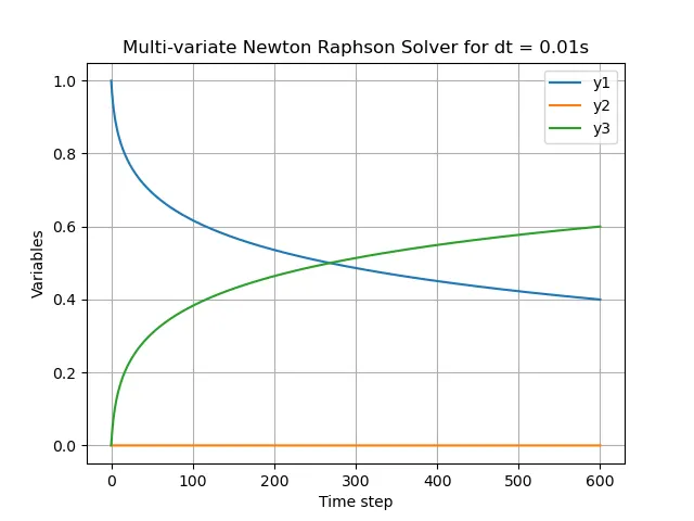
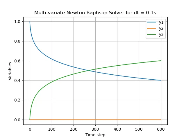
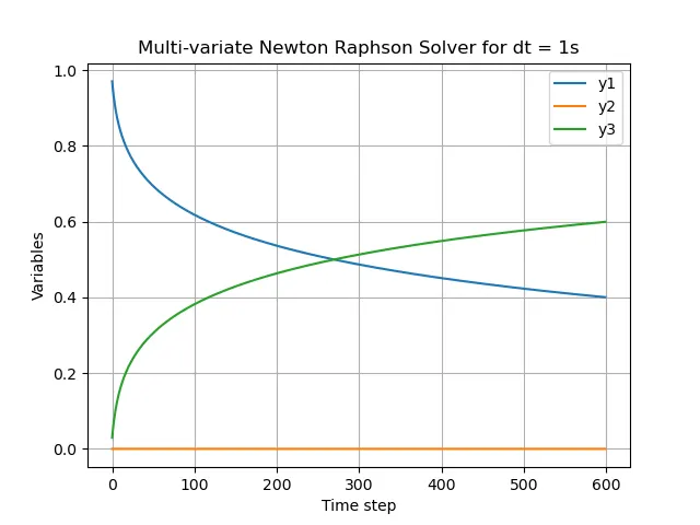
Upon comparision of different values of dt on the solution method, it is quite evident that there is little to no variation in the final results, so in order to save the computational resources, the maximum value of dt can be choosen.