Week 6 - Multivariate Newton Rhapson Solver

Multivariate Newton Rhapson Solver

• Aim :

1. Solving the given equations using multivariate Newton Raphson method with implicit or Backward Differencing scheme.
2. Explain the ideal step size for this case.

• Theory :

Equations we have to solve are given as follows:

`(dy_1/dt) = -0.04*y_1 + 10^4*y_2*y_3`

`(dy_2/dt) = 0.04*y_1-10^4*y_2*y_3-3.10^7*y_2^2`

`(dy_3/dt) = 3.10^7*y_2^2`

Multi-variate Newton Raphson Method - 

The Newton-Raphson method (also known as Newton's method) is a way to quickly find a good approximation for the root of a real-valued function f(y) = 0. It uses the idea that a continuous and differentiable function can be approximated by a straight line tangent to it. Suppose you need to find the root of a continuous, differentiable function f(y), and you know the root you are looking for is near the point y = `y_old`​. Then Newton's method tells us that a better approximation for the root is 

`y_(New) = y_(Old) -[ f(y_Old)]/[f'(y_old)]`

Multi-variate Newton Raphson Method is used when the equations are coupled and non linear. The equations are solved by forming matrices as there are multiple variables in equations.

It is given by,

`Y^( New) = Y^(old ) - alpha*J^(-1)*F`

where, `Y^(New)` is the value of X at next time step

          `Y^(old)` is the value of X at current time step

           alpha is the relaxation factor

           J is the jacobian matrix

           F is the function matrix 

Matrices of the above given equation are given as,

`Y^(New) = [(y_1^(New)),(y_2^(New)),(y_3^(New))]`

`Y^(old) = [(y_1^(old)),(y_2^(old)),(y_3^(old))]`

`J = [((df_1)/dy_1, (df_1)/dy_2,(df_1)/dy_3),((df_2)/dy_1,(df_2)/dy_2,(df_2)/dy_3),((df_3)/dy_1,(df_3)/dy_2,(df_3)/dy_3)]`

`F = [(f_1),(f_2),(f_3)]`

Backward Differencing Method - 

Implicit scheme or backward differencing method is given by,

`f^'(y_i) = (f(y_i) - f(y_(i-1)))/(dy)`

Considering general equation,

`dy/dt = f(y_i)`

`(y_i^n - y_i^(n-1))/(dt) = f(y_i)`

`y_i^(n-1) +f(y_i)*dt -y_i^n = 0`

Now considering our equation from the problems,

`f1 = y_1^(old )+ dt*(-0.04*y_1^(New) + 1e4*y_2*y_3) - y_1^(New)`

`f2 = y_2^(old) + dt*(0.04*y_1 - 1e4*y_2^(New)*y3 - 3e7*y_2^(New)*y_2^(New)) - y_2^(New)`

`f3 = y_3^(old) + dt*(3e7*y2*y2) - y_3^(New)`

• Code :

import math
import matplotlib.pyplot as plt
import numpy as np
from numpy.linalg import inv

def f1(y1_old, y1, y2, y3, dt):
	return y1_old + dt*(-0.04*y1 + 1e4*y2*y3) - y1

def f2(y2_old, y1, y2, y3, dt):
	return y2_old + dt*(0.04*y1 - 1e4*y2*y3 - 3e7*y2*y2) - y2

def f3(y3_old, y1, y2, y3, dt):
	return y3_old + dt*(3e7*y2*y2) - y3

def jacobian(y1_old, y2_old, y3_old, y1, y2, y3, dt):

	J = np.ones((3,3))
	dy = 1e-8

	#Row 1
	J[0,0] = (f1(y1_old, y1+dy, y2, y3, dt) - f1(y1_old, y1, y2, y3, dt))/dy
	J[0,1] = (f1(y1_old, y1, y2+dy, y3, dt) - f1(y1_old, y1, y2, y3, dt))/dy
	J[0,2] = (f1(y1_old, y1, y2, y3+dy, dt) - f1(y1_old, y1, y2, y3, dt))/dy

	#Row 2
	J[1,0] = (f2(y2_old, y1+dy, y2, y3, dt) - f2(y2_old, y1, y2, y3, dt))/dy
	J[1,1] = (f2(y2_old, y1, y2+dy, y3, dt) - f2(y2_old, y1, y2, y3, dt))/dy
	J[1,2] = (f2(y2_old, y1, y2, y3+dy, dt) - f2(y2_old, y1, y2, y3, dt))/dy

	#Row 3
	J[2,0] = (f3(y3_old, y1+dy, y2, y3, dt) - f3(y3_old, y1, y2, y3, dt))/dy
	J[2,1] = (f3(y3_old, y1, y2+dy, y3, dt) - f3(y3_old, y1, y2, y3, dt))/dy
	J[2,2] = (f3(y3_old, y1, y2, y3+dy, dt) - f3(y3_old, y1, y2, y3, dt))/dy
	return J



t_0 = 0
t_end = 6000
dt = 0.1
t = np.arange(t_0, t_end)
time = len(t)

#initial guess value
y1 = 1
y2 = 0
y3 = 0

#new guess values
y1_new = []
y2_new = []
y3_new = []

for i in range(1, time+1):

	alpha = 1
	error = 9e9
	tol = 1e-6
	#numpy column vector
	Y_old = np.ones((3,1))
	Y_old[0] = y1
	Y_old[1] = y2
	Y_old[2] = y3

	#guess values
	y_guess = np.ones((3,1))
	y_guess[0] = y1
	y_guess[1] = y2
	y_guess[2] = y3

	#numpy column vector for F
	F = np.ones((3,1))

	#newton raphson method loop
	iter = 0

	while error > tol:
		#Jacobian using numerical method
		J = jacobian(Y_old[0], Y_old[1], Y_old[2], y_guess[0], y_guess[1], y_guess[2], dt)

		#computing F vector 
		F[0] = f1(Y_old[0], y_guess[0], y_guess[1], y_guess[2], dt)
		F[1] = f2(Y_old[1], y_guess[0], y_guess[1], y_guess[2], dt)
		F[2] = f3(Y_old[2], y_guess[0], y_guess[1], y_guess[2], dt)

		#computing new values
		y_new = y_guess - alpha*np.matmul(inv(J), F)

		#computing max abs error
		error = np.max(np.abs(y_new - y_guess))
		print(error)

		#updating old values
		y_guess = y_new;

		#log message
		log_message = 'iteration # = {0} y1 = {1} y2 ={2} y3 = {3}'.format(iter, y_new[0], y_new[1], y_new[2])
		print(log_message)
		iter = iter + 1

	#final results
	
	y1 = y_new[0]
	y2 = y_new[1]
	y3 = y_new[2]
	

	y1_new.append(y_new[0])
	y2_new.append(y_new[1])
	y3_new.append(y_new[2])

#plotting figures
plt.plot(t, y1_new)
plt.plot(t, y2_new)
plt.plot(t, y3_new)
plt.xlabel("Simulation time in sec")
plt.ylabel("Y_new")
plt.legend(['Y1', 'Y2', 'Y3'])
plt.title("Multivariate newton Raphson method")
plt.show()

Plots :

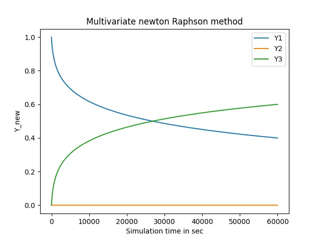
1. When time step = 0.01

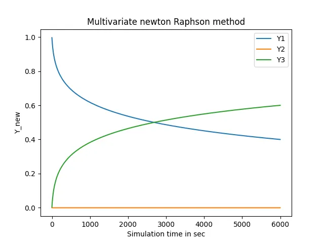
2. When time step = 0.1

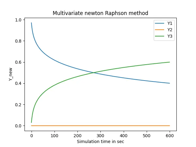
3. When time step = 1

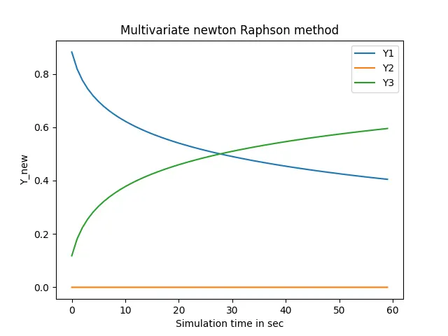
4. When time step = 10

• Choosing the ideal Time step :

The simulation is ran for four time steps. As observed, the graphs look similar for all the cases and values of y1, y2 and y3 are also close to each other in all the cases. As we reduce the value of time step, we get more accurate results. But the simulation time also increases for smaller time steps. So choosing a right time step comes down to preference of accuracy or speed. 

For me ideal time step in this case would be 0.1 as both fairly accurate results and fast calculations are achieved.