Week 6 - Multivariate Newton Rhapson Solver

Multivariate Newton Rapshon Method :-
In numerical analysis, Newton's Method also known as the Newton-Raphson method is a root.
Finding algorithms that produce a successively better approximation to the root or zeros of a real values function.
The most basic version starts with a single variable function defined for a real variable x, the function f defined for a real variable x,
the function f', and an initial guess for the root of f.
The idea is to start with an initial guess which is reasonably close to the true root, then to approximate the function by its tangent
line using calculus, and finally to compute the x-intercept of its tangent line by elementary algebra.

This x-intercept will typically be a better approximation to the original function root than the first guess, and the method can be iterated.

To find Jacobian Matrix
Since we have three equation and three variable. Therefore, there will be three rows and columns respectively.
Here,
yn2−yn−12=0.04yn1−104yn2yn3−3⋅107(yn2)2
dy3dt=3⋅107⋅(yn2)2
fn1=yn1+△t(0.04yn1−104yn2yn3)−yn−11=0
fn2=yn2−△t(0.04yn1−104yn2yn3−3⋅107(yn2)2)−yn−12=0
fn3=yn3−△t(3⋅107(yn2)2)−yn−13=0
J=⎡⎢ ⎢ ⎢ ⎢ ⎢ ⎢⎣∂fn1/∂yn1 ∂fn1/∂yn2 ∂fn1/∂yn3; ∂fn2/∂yn1 ∂fn2/∂yn2 ∂fn2/∂yn3; ∂fn3/∂yn1 ∂fn3/∂yn2 ∂fn3/∂yn3⎤⎥ ⎥ ⎥ ⎥ ⎥ ⎥⎦
y(new)n=ynold+α[(J−1)F]n
F=⎡⎢⎣f1 f2 f3⎤⎥⎦

Python Code -

"""
Program to solve the coupled non linear equation
by Saurabh Nambiar
"""
import numpy as np
from numpy.linalg import inv
import matplotlib.pyplot as plt
# Time Interval
t_start = 0
t_end = 600
n = 60000
dt = (t_end - t_start)/n
iteration = 0
# Initial Guess Value
y1 = 1
y2 = 0
y3 = 0
# Equation
def f1(y1_old,y2_old,y3_old,y1,y2,y3,dt):

	return y1_old + (-0.04*y1 + pow(10,4)*y2*y3)*dt - y1
def f2(y1_old,y2_old,y3_old,y1,y2,y3,dt):

	return y2_old + (0.04*y1 - pow(10,4)*y2*y3 - 3*pow(10,7)*y2*y2)*dt - y2
def f3(y1_old,y2_old,y3_old,y1,y2,y3,dt):

	return y3_old + (3*pow(10,7)*y2*y2)*dt - y3
# Jacobian Matrix
def jacobian(y1_old,y2_old,y3_old,y1,y2,y3,dt):
	J = np.zeros((3,3))
	h = 1e-5
# First Row
	J[0,0] = (f1(y1_old,y2_old,y3_old,y1+h,y2,y3,dt)-f1(y1_old,y2_old,y3_old,y1,y2,y3,dt))/h
	J[0,1] = (f1(y1_old,y2_old,y3_old,y1,y2+h,y3,dt)-f1(y1_old,y2_old,y3_old,y1,y2,y3,dt))/h
	J[0,2] = (f1(y1_old,y2_old,y3_old,y1,y2,y3+h,dt)-f1(y1_old,y2_old,y3_old,y1,y2,y3,dt))/h
# Second Row
	J[1,0] = (f2(y1_old,y2_old,y3_old,y1+h,y2,y3,dt)-f2(y1_old,y2_old,y3_old,y1,y2,y3,dt))/h
	J[1,1] = (f2(y1_old,y2_old,y3_old,y1,y2+h,y3,dt)-f2(y1_old,y2_old,y3_old,y1,y2,y3,dt))/h
	J[1,2] = (f2(y1_old,y2_old,y3_old,y1,y2,y3+h,dt)-f2(y1_old,y2_old,y3_old,y1,y2,y3,dt))/h
# Third Row
	J[2,0] = (f3(y1_old,y2_old,y3_old,y1+h,y2,y3,dt)-f3(y1_old,y2_old,y3_old,y1,y2,y3,dt))/h
	J[2,1] = (f3(y1_old,y2_old,y3_old,y1,y2+h,y3,dt)-f3(y1_old,y2_old,y3_old,y1,y2,y3,dt))/h
	J[2,2] = (f3(y1_old,y2_old,y3_old,y1,y2,y3+h,dt)-f3(y1_old,y2_old,y3_old,y1,y2,y3,dt))/h
	return J
# Newton Rhaphson Method
def Newton_Rhaphson(y1,y2,y3,y1_guess,y2_guess,y3_guess,dt):
# Vector Equation
	global iteration

	global iteration
	Y_old = np.zeros((3,1))
	Y_old[0] = y1_guess
	Y_old[1] = y2_guess
	Y_old[2] = y3_guess
#print(Y_old)
	F = np.zeros((3,1))
# Solver Parameter
	error = 9e9
	tol = 1e-4
	alpha = 1
#iter = 0
	while(error>=tol):
# Jacobi set for the equation
		iteration = iteration + 1
		J = jacobian(y1,y2,y3,Y_old[0],Y_old[1],Y_old[2],dt)
		F[0] = f1(y1,y2,y3,Y_old[0],Y_old[1],Y_old[2],dt)
		F[1] = f2(y1,y2,y3,Y_old[0],Y_old[1],Y_old[2],dt)
		F[2] = f3(y1,y2,y3,Y_old[0],Y_old[1],Y_old[2],dt)
		Y_new = Y_old - alpha*(np.matmul(inv(J),F))
		error = np.max(np.abs(Y_new-Y_old))
		print(error,tol)
		Y_old = Y_new
#print(iter)
		log_message = 'iteration = {0} y1 = {1} y2 = {2} y3 = {3}'.format(iteration,Y_new[0],Y_new[1],Y_new[2])
		print(log_message)
#iter = iter + 1
	return [Y_new[0],Y_new[1],Y_new[2]]
# Implicit Euler
def implicit(y1,y2,y3,t_start,t_end,dt):
	t = np.arange(t_start,t_end,dt)
	time = len(t)
	Y_1 = np.zeros(time)
	Y_2 = np.zeros(time)
	Y_3 = np.zeros(time)
	Y_1[0] = y1
	Y_2[0] = y2
	Y_3[0] = y3
	y1_guess = 0
	y2_guess = 0
	y3_guess = 0
	for i in range (1,time):
		Y_1[i],Y_2[i],Y_3[i] = Newton_Rhaphson(Y_1[i-1],Y_2[i-1],Y_3[i-1],y1_guess,y2_guess,y3_guess,dt)
		y1_guess = Y_1[i]
		y2_guess = Y_2[i]
		y3_guess = Y_3[i]
	return [t,Y_1,Y_2,Y_3]
t, y1, y2, y3 = implicit(1,0,0,0,600,0.1)
plt.plot(t,y1)
plt.plot(t,y2)
plt.plot(t,y2)
plt.plot(t,y3)
plt.xlabel('Simulation Time (sec)')
plt.ylabel('Variable')
plt.legend(['y1','y2','y3'])
plt.title('Multivarient Newton Ranpshon Method for dt = 0.01')
plt.grid('on')
plt.show()

Results-

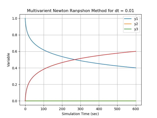
Choosing a suitable time step size:-

• The simulation has been run for three different time steps that 0.1,1 and 0.01 respectively.
  But there is not much change in the graph
• 
  There is no effect of the time step on the simulation because we have an implicit method and if we have used the explicit it will get
  effect due to time step.
• 
  However, the implicit method is difficult to code a certain extend as compared to explicit.
• 
  But for choosing a suitable time step size we can conclude that the time step of 0.01 is suitable because the Number of iteration is
  more, more iteration there will be more accuracy in the solution.
• 
  Hence, a time step size of 0.01 is the ideal time step size.