Week 6 - Multivariate Newton Rhapson Solver

In the CFD domain, most of the heat transfer or fluid mechanics equations when discretised yield linear or non-linear system of equations depending upon the nature of partial differential equation they are derived from.

When dealing with equations which are tightly coupled and linear in nature, finding a solution using a simultaneous approach or direct methods like Gauss elimination, LU decomposition or cyclic reduction works best.
However, when equations are complex and non-linear in nature solving them computationally becomes expensive. Hence, in such cases it is preferable to treat each equation as if it has only single unknown, temporarily treating the other variables as known, using the best current available values(often loosely termed as guess values or initial values) for them.
These equations are in turn solved in successive iterations until values for unknowns are satisfied.

While solving these equations the coefficients and source terms that depend on other variables changes as the computation proceeds, hence it is inefficient to solve the equations accurately in each iteration.
Owning to this direct solvers are rarely used and rather iterative solvers are preferred. Here, iterations performed on each equation are called as inner iterations.

Further, in order to obtain the values of unknowns till all equations are satisfied the above iterations are performed and after each iteration, the source vector must be updated and the cycles continue. These cycles are called as outer
iterations.

Optimisation of the above-mentioned process requires pre-hand knowledge of the number of inner iterations required per each outer iteration. Controlling the change in the value of each variable is necessary to avoid divergence or to avoid artificial errors or numerical errors.
Unfortunately, it is very difficult to analyse the convergence of these methods hence the selection of relaxation factor to control the variation in variables is mostly empirical. These types of multigrid solutions can also be applied to coupled systems.

To solve non-linear equations there are mainly two numerical approaches:
a. Newton-like techniques
b. Global techniques.

Newton-like techniques are faster comparatively when they have a good estimation of the solution is available; however, they tend to diverge, which is an advantage in the latter technique. Hence, a combination of both is generally used industry-wide to obtain fast and converging results on a non-linear coupled system of equations.

Let `x_0` be an approximate root of the equation `f(x)=0`. If `x_1 = x_0 + h` be the exact root, then `f(x_1)=0`.

expanding `f(x_0 + h)` using Taylor's series we get,
`f(x_0 + h) = f(x_0) + hf'(x_0) + h^2/2 f''(x_0) + ... = 0`
Since `h` is small neglecting higher powers of `h^2` and higher powers of `h`, we get
`f(x_0) + hf'(x_0) = 0`
`or, h = - (f(x_0))/(f'(x_0))`
`x_1 - x_0 = - (f(x_0))/(f'(x_0))`
`x_1 = x_0 - (f(x_0))/(f'(x_0))`

Similarly if we start with `x_1` as approximation we get `x_2`, which can be written as
`x_2 = x_1 - (f(x_1))/(f'(x_1))`
Therefore, we can write in general,

`x_n+1 = x_n - (f(x_n))/(f'(x_n))`

which is known as Newton-Rhapson or Newton iteration formula.

This iteration is continued until the difference `x_(n+1) - x_n` reduces to the desired level. This method can be roughly equated to curve approximation. In Newton-Rhapson when the estimate is close enough to the root, the method converges quadratically i.e. the error at iteration `n+1` is proportional to the square of the error at iteration n. This means that error at iteration `n+1` is proportional to the square of the error at iteration `n`.

For generic system of equations written as :
`f_i(x_1,x_2,x_3,...x_n) = 0 `
The method is extended to system of equations by using Taylor's series for multiple equations:
`f_i(x_1,x_2, x_3, ... x_n) = f_i(x_1^k + x_2^k + x_3^k ... x_n^k) + \sum(x_j^(k+1) - x_j^k) df(x_1^k, x_2^k, x_3^k, ... x_n^k)/dx_n`
These set of equations are set to zero to get a system of equations which can be solved by direct methods like Gauss Elimination or such.


The matrix of the system is set of partial differential derivatives:
`a_(ij) = df_i(x_1^k, x_2^k, x_3^k, ... x_n^k)/dx_j`
`i=1, 2, 3, ..n;` `j = 1, 2, 3...n`
this matrix is Jacobian of the system.
The system of equations is :
`sum_(j=1)^n a_(ij)( x_j^(k+1) - x_j ) = -f_i( x_1^k,x_2^k,x_3^k,....x_n^k)`

The code will try to solve the given system of coupled equations.
The code has three functions namely f1, f2 and f3 which will return terms accumulated to either side of equality sign.
Function jacobian to evaluate the jacobian matrix and two utility functions (check_create_path & create_log_handler) for assisting the monitoring and storing intermediate data generated during script execution.

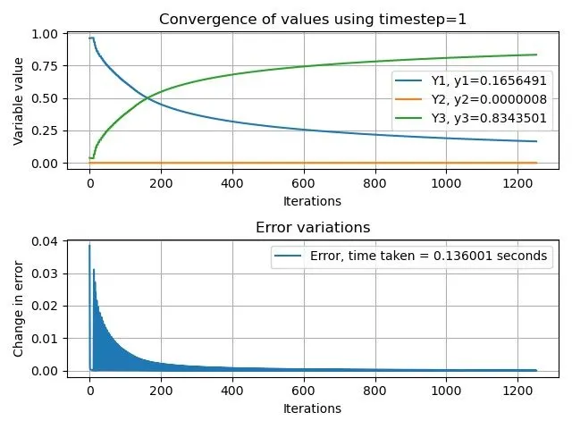
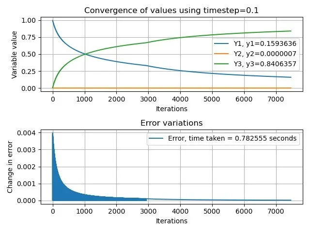
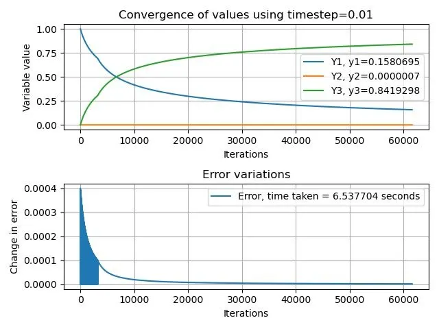
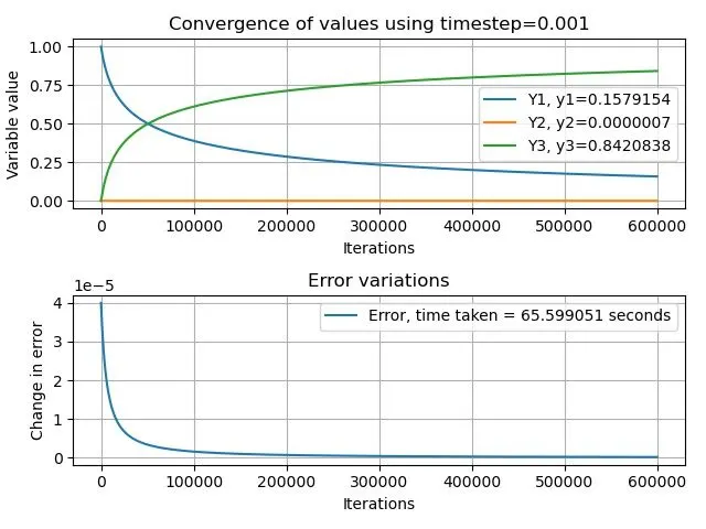
The whole process of using initial guess values repeats for four different time steps. In each time step, the equations are solved and updated till they converge to the desired tolerance level of `1e-4`.
When such a step is achieved the loop moves to next time step iteration and repeats the process. In the end, the values of variables and errors calculated during each iteration are collected and plotted to observe the change in variables over the iterations.

As mentioned earlier, if the estimate is closer to the root, the solution converges quickly. However, when large systems are solved two challenges are presented.
1. The Jacobian matrix is evaluated at each inner iteration which is expensive computationally as there are `n^2` elements in the matrix.
2. The next is that a direct method of Jacobian calculation may not exist and often for implicit equations or systems complicated in nature, differentiation maybe impossible.

                                Case1      Case2      Case3      Case4       Case5
Step Size                           1        0.1       0.01      0.001      0.0001
No of time steps                  600       6000      60000     600000     6000000
Y1 converged                0.1656491  0.1593636  0.1580695  0.1579154   0.1578998
Y2 converged                0.0000008  0.0000007  0.0000007  0.0000007   0.0000007
Y3 converged                0.8343501  0.8406357  0.8419298  0.8420838   0.8420995
Time Taken                   0.136001   0.782555   6.537704  65.599051  654.492486
Diff % with case              0.77494    0.14638    0.01697    0.00157           0
having highest accuracy

Case1

Case2

Case3

Case4

Case5

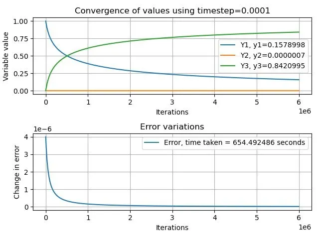
• The solution converges quickly for bigger step size(Case1) value as there are less inner iterations(no of time steps) to loop through as compared to Case5 where no of time steps are more.
• However, accuracy tends to be less when the step size is large. This can again be observed in Case1 vs Case5, where Case5 having smallest step size has the best accuracy as compared to other cases.
• Owning to more number of time steps the computation becomes expensive in nature. Hence, a trade-off has to be made between computational efforts vs accuracy of the solutions.
• Observing the above table both Case3 and Case4 can be considered as optimum solutions for the given set of equations considering both computational efforts and accuracy.