Week 6 - Multivariate Newton Rhapson Solver

MULTIVARIANTE NEWTON RHAPSON SOLVER

Objective: solving three non-linear coupled equations using implicit Euler Method/Backward Differencing of multivariate Newton-Rhapson solver.

Set of three equations as follows:

Rearranging the above equations and assigning each to a function.

`f_1 = y_1old +(-0.04y_1 + 10^4y_2y_3)dt-y_1`

`f_2 = y_2old+(0.04y_1-10^4y_2y_3-3*10^7y_2^2)dt-y_2`

`f_3 = y_3old+3.10^7y_2^2dt-y_3`

`:. dy/dt = (y-yold)/dt`

multivariate Newton Rhapson formula:

`y_n = y_(n-1) -alpha.J^-1F`

J = jacobian matrix(3*3)

J = `[[(df_1)/dy_1,(df_1)/dy_2,(df_1)/dy_3],[(df_2)/dy_1,(df_2)/dy_2,(df_2)/dy_3],[(df_3)/dy_1,(df_3)/dy_2,(df_3)/dy_3]]`

F = `[[f_1],[f_2],[f_3]]`

Below is the python program to written to solve the above equations.

"""
Pyhton Program is written to solve the non-linear coupled equation by using multivariant newton raphson technique

Three non-linear coupled equations are taken and are assigned to functions f1,f2,f3.
"""
import matplotlib.pyplot as plt 
import numpy as np 
from numpy.linalg import inv

# Equation
def f1(y1_old,y1,y2,y3,dt): #dy1/dt = -0.04*y1 + pow(10,4)*y2*y3
	
	return y1_old - 0.04*y1*dt + pow(10,4)*y2*y3*dt - y1

def f2(y2_old,y1,y2,y3,dt): #dy2/dt = 0.04*y1 - pow(10,4)*y2*y3 - 3*pow(10,7)*y2*y2
	
	return y2_old + 0.04*y1*dt - pow(10,4)*y2*y3*dt - 3*pow(10,7)*pow(y2,2)*dt - y2

def f3(y3_old,y1,y2,y3,dt): #dy3/dt = 3*pow(10,7)*y2*y2
	
	return y3_old + 3*pow(10,7)*pow(y2,2)*dt - y3

# Jacobian Matrix
def jacobian(y1_old,y2_old,y3_old,y1,y2,y3,dt):
	
	J = np.ones((3,3))
	#step size
	h = 1e-5
	# First Row
	J[0,0] = (f1(y1_old,y1+h,y2,y3,dt)-f1(y1_old,y1,y2,y3,dt))/h
	J[0,1] = (f1(y1_old,y1,y2+h,y3,dt)-f1(y1_old,y1,y2,y3,dt))/h
	J[0,2] = (f1(y1_old,y1,y2,y3+h,dt)-f1(y1_old,y1,y2,y3,dt))/h

	# Second Row 
	J[1,0] = (f2(y2_old,y1+h,y2,y3,dt)-f2(y2_old,y1,y2,y3,dt))/h
	J[1,1] = (f2(y2_old,y1,y2+h,y3,dt)-f2(y2_old,y1,y2,y3,dt))/h
	J[1,2] = (f2(y2_old,y1,y2,y3+h,dt)-f2(y2_old,y1,y2,y3,dt))/h

	# Third Row
	J[2,0] = (f3(y3_old,y1+h,y2,y3,dt)-f3(y3_old,y1,y2,y3,dt))/h
	J[2,1] = (f3(y3_old,y1,y2+h,y3,dt)-f3(y3_old,y1,y2,y3,dt))/h
	J[2,2] = (f3(y3_old,y1,y2,y3+h,dt)-f3(y3_old,y1,y2,y3,dt))/h

	return J

# Time Interval
time = 600
dt = 0.001
n = int(time/dt)
# Initial Guess Value
y1_old = 1
y2_old = 0
y3_old = 0

Y_old = np.ones((3,1))
Y_old[0] = y1_old
Y_old[1] = y2_old
Y_old[2] = y3_old

F = np.copy(Y_old)

# Solver Parameter
y1 = []
y2 = []
y3 = []
iteration = []
t = 1 #iterations

for i in range(0,n):
	error = 9e9
	tol = 1e-6
	alpha = 1

	while error>tol:

		J = jacobian(y1_old,y2_old,y3_old,Y_old[0],Y_old[1],Y_old[2],dt)

		F[0] = f1(y1_old,Y_old[0],Y_old[1],Y_old[2],dt)
		F[1] = f2(y2_old,Y_old[0],Y_old[1],Y_old[2],dt)
		F[2] = f3(y3_old,Y_old[0],Y_old[1],Y_old[2],dt)

		Y_new = Y_old - alpha*np.matmul(inv(J),F)
		
		error = np.max(np.abs(Y_new-Y_old))
		
		Y_old = Y_new
		
	log_message = 'iteration = {0} y1 = {1} y2 = {2} y3 = {3}'.format(t,Y_new[0],Y_new[1],Y_new[2])
	
	print(log_message)
		
	t = t + 1

	y1.append(Y_new[0])
	y2.append(Y_new[1])
	y3.append(Y_new[2])			
	iteration.append(t)
	
	Y_old = Y_new
	y1_old = Y_new[0]
	y2_old = Y_new[1]
	y3_old = Y_new[2]

plt.plot(iteration,y1)
plt.plot(iteration,y2)
plt.plot(iteration,y3)
plt.xlabel('time:'+ str(dt*n))
plt.ylabel('Variable')
plt.legend(['y1','y2','y3'])
plt.title('Multivarient Newton Ranpshon Method for:'+str(dt))
plt.grid('on')
plt.show()

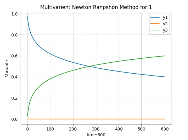
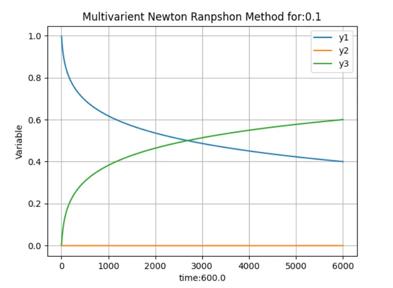
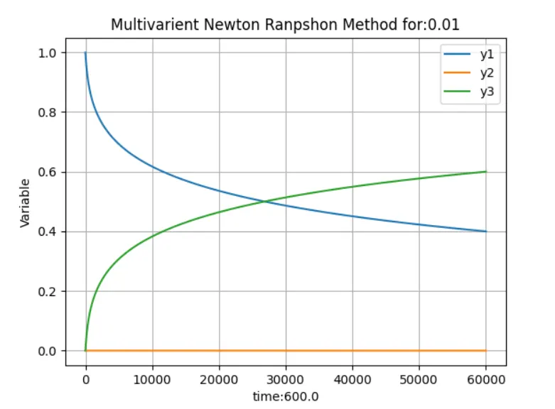
Results: Plots obtained for various timestep sizes are as follows.

1.Time = 600 sec, dt = 1, n = 600

2.Time = 600 sec, dt = 0.1, n = 6000

3.Time = 600 sec, dt = 0.01, n = 60000

4.Time = 600 sec, dt = 0.001, n = 600000

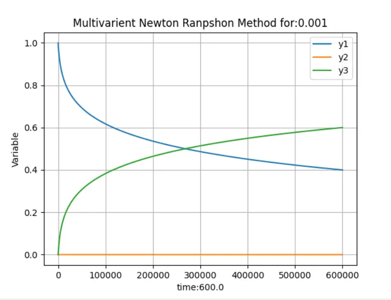
From the above graphs, it is clear that irrespective the timestep sizes end result remained same, this is due to use of Implicit method which is very stable in every timestep given.

Choose a suitable step size and explain the reason for choosing that step size, what is the ideal step size in this case?

• Use of implicit method to solve the non-linear coupled equations helped in maintaining the stability of the solution irrespective of the timestep size.
• Time step size 1,0.1,0.01,0.001 has yielded identical results.
• Choosing a suitable step doesn't mean any thing in implicit method because of its robustness.
• However ideal step size can be 0.1 or 0.01, since this two sizes gave similar results and the computional time taken is less than a minute.
• Implicit method is a complex method, and requires high computational power which provides with accurate results, so choosing the suitable timestep depends computational efficiency.