Week 6 - Multivariate Newton Rhapson Solver

OBJECTIVES :- To solve given equations of ODE by using Multivariate Newton Rhapson solver.

PROBLEM STATEMENT :-

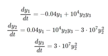
By solving above ODE, we need to find following points-

• Jacobian should be estimated numerically
• Solve the problem by using Implicit Euler method/Backward differencing.
• Choose suitable step size and explain the reason for choosing that time step size, what is the ideal step size in this case?
• Write the code and results.

INTRODUCTIONS & THEORY :-

In first year calculus, most students learn Newtons method for solving non linear equations f(x) = 0, which iteratively improves a sequence of guesses for the solution x by approximating f by a straight line. That is, is approximates a nonlinear equation by a sequence of approximate linear equations.

This can be extend to systems of nonlinear equations as a multidimensional Newton method, in which we iterate by solving sequence of linear (matrix) system of equations. This is one example of an amazing fact: linear algebra is a fundamental tool even for solving nonlinear equations.

APPLICATIONS :-

• Minimization & maximization problem
• Multiplicative inverses of numbers and power series
• Solving transcendental equations
• Obtaining zeros of special functions
• Numerical verification for solutions of non linear equations
• CFD modeling

Multivariate Newton Rahpson Solver :-

We observe the avove system are three non-linear coupled equations. Do we establish why they are coupled? because of these equations (y1, y2, y3) can be solved by solving the three equations together. We can say these equations are non-linear because of the unknown elements which we are going to solve multiply themselves.

Here the Newton Rahpson solver is impemented to solve the non-linear system of coupled equations at each time step using an implicit method.

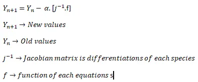
Here, the Jacobian matrix cantains the differentiation of the net rate of reaction of each unknown value.

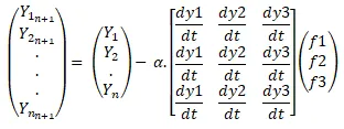
In this challenge solving jacobian matrix using numerical method not analytical.

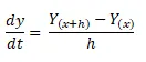
The principle of jacobian matrix Numerical as forwarding difference method,

.

Implicit solver :-

Here, we are initializing the ODE in the form of-

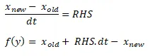
We have written system of non-linear equations in the form of implicit

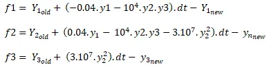
Now we are going to solve Multivariate Newton Raphson method,

here initial values taken

y1 = 1

y2 = 0

y3 = 0, and update each time step from ynew values.

STEP WISE PROCEDURES :-

1. Import numpy for solving ODE’s.
2. Import inverse (i.e. inv) for taking inverse of jacobian matrix
3. Import matplotlib to plot each ODE equation.
4. Define each one non-linear equations which are the combinations of old value, y1, y2, y3 & dt.
5. Return in the sense to solve at each time steps
6. Define jacobian matrix of all the non-linear parameters.
7. Here we have three unknown and three equations so according to that we need total 9 rows after derivating of each functions.
8. First differentiate with y1, then y2 and then y3 likewise.
9. Define step size in the range of 0 to 600 time by taking step size equal to 0.5.
10. Define initial guess values i.e. y1=1, y2=0 & y3=0.
11. Define the final guess values in which we appended the y_new values i.e. “y_new = y_guess – alpha*(abs(y_new – y_guess))”
12. Use the for loop for time range from 1 to 600.
13. Define error, tolerance and alpha values.
14. Update old values & guess values which are 3 by 1 size matrix.
15. Use the newton rahpson method by computing “error> tol” in while loop.
16. Use the jacobian formula & computing the F vector.
17. Computing new values, maximum absolute error & update old values i.e. guess values.
18. Log the message to showing the number of iterations required to converge the solutions.
19. Plot figure for each new value vs time.

PYTHON CODE :-

"""
Program to solve the system of coupled non-linear equations
(-0.04*y1) + 1e4*y2*y3 = dy1/dt
(0.04*y1) - 1e4*y2*y3 - 3e7*y2**2 = dy2/dt
3e7*y2**2 = dy3/dt

Modules required
1. numpy is required for matrix multiplications
2. inv is required for computing the inverse of a matrix
"""
import numpy as np 
from numpy.linalg import inv 
import matplotlib.pyplot as plt 

def f1(y1_old, y1, y2, y3, dt):
	#First non-linear equation
	return y1_old + dt*(-0.04*y1 + pow(10,4)*y2*y3) - y1

def f2(y2_old, y1, y2, y3, dt):
	#Second non-linear equation
	return y2_old + dt*(0.04*y1 - pow(10,4)*y2*y3 -3*pow(10,7)*pow(y2,2)) - y2

def f3(y3_old, y1, y2, y3, dt):
	#Third non-linear equation
	return y3_old + dt*(3*pow(10,7)*pow(y2,2)) - y3

def jacobian(y1_old, y2_old, y3_old, y1, y2, y3, dt):
	# Defining the jacobian

	# 3 by 3 unit matrix
	J = np.ones((3, 3))
	d = 1e-8

	#Derivative of each function
	# Row-1
	J[0,0] = (f1(y1_old, y1+d, y2, y3, dt) - f1(y1_old, y1, y2, y3,dt))/d
	J[0,1] = (f1(y1_old, y1, y2+d, y3, dt) - f1(y1_old, y1, y2, y3, dt))/d
	J[0,2] = (f1(y1_old, y1, y2, y3+d, dt) - f1(y1_old, y1, y2, y3, dt))/d

	# Derivative of second function
	# Row-2
	J[1,0] = (f2(y2_old, y1+d, y2, y3, dt) - f2(y2_old, y1, y2, y3, dt))/d
	J[1,1] = (f2(y2_old, y1, y2+d, y3, dt) - f2(y2_old, y1, y2, y3, dt))/d
	J[1,2] = (f2(y2_old, y1, y2, y3+d, dt) - f2(y2_old, y1, y2, y3, dt))/d

	# Derivative of third function
	# Row-3
	J[2,0] = (f3(y3_old, y1+d, y2, y3, dt) - f3(y3_old, y1, y2, y3, dt))/d
	J[2,1] = (f3(y3_old, y1, y2+d, y3, dt) - f3(y3_old, y1, y2, y3, dt))/d
	J[2,2] = (f3(y3_old, y1, y2, y3+d, dt) - f3(y3_old, y1, y2, y3, dt))/d
	return J

# Step size (loop)
t_start = 0
t_end = 600
dt = 0.5
t = np.arange(t_start, t_end)
time = len(t)

# Defining the initial guess values
y1 = 1
y2 = 0
y3 = 0

# Defining the final guess values
y1_new = []
y2_new = []
y3_new = []

for i in range(1, time+1):

	#Initial error
	error = 9e9
	tol = 1e-6
	alpha = 1

	# numpy column vector (Update old values)
	Y_old = np.ones((3,1))
	Y_old[0] = y1
	Y_old[1] = y2
	Y_old[2] = y3

	# Guess values
	y_guess = np.ones((3,1))
	y_guess[0] = y1
	y_guess[1] = y2
	y_guess[2] = y3

	# numpy column vector for F
	F = np.ones((3,1))

	# Starting the newton raphson method loop
	iter = 0
	while error > tol:
		#Computing the jacobian old values are used
		# Jacobian using numerical method
		J = jacobian(Y_old[0], Y_old[1], Y_old[2], y_guess[0], y_guess[1], y_guess[2], dt)

		# Computing the F vector - old values are used
		F[0] = f1(Y_old[0], y_guess[0], y_guess[1], y_guess[2], dt)
		F[1] = f2(Y_old[1], y_guess[0], y_guess[1], y_guess[2], dt)
		F[2] = f3(Y_old[2], y_guess[0], y_guess[1], y_guess[2], dt)

		#Computing new values
		y_new = y_guess - alpha*np.matmul(inv(J), F)

		# Computing max abs error
		error = np.max(np.abs(y_new - y_guess))
		print(error)

		# Updating old values 
		y_guess = y_new

		#log message
		log_message = 'iteration # = {0} y1 = {1} y2 = {2} y3 = {3}'.format(iter, y_new[0], y_new[1], y_new[2])
		print(log_message)
		iter = iter + 1

	# Final results
	y1 = y_new[0]
	y2 = y_new[1]
	y3 = y_new[2]

	y1_new.append(y_new[0])
	y2_new.append(y_new[1])
	y3_new.append(y_new[2])

# Plotting figures
plt.plot(t, y1_new)
plt.plot(t, y2_new)
plt.plot(t, y3_new)
plt.xlabel("Simulation time (sec)")
plt.ylabel("Y_new")
plt.legend(['Y1','Y2','Y3'])
plt.title("Multivariate newton Raphson Method")
plt.savefig("Multivariate Numerical Raphson Method")
plt.show()

Reason behind using this step size :-

As we need converge solution and for that we need to fix the time range. So here I fixed the time range from 1 to 600 sec. To simulate this time range we need time step size so that time should be equally distributed. This time step is for converging the solution within given time range.

It might be the ideal time step, but we can put different time step as well according to our convenience. But, if we shouldn't consider time range then our solution runs upto it's error reaches.

RESULTS :-

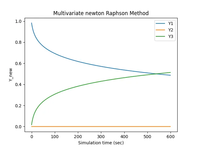
As we have seen the above results approximation of unknown values y1, y2 & y3 using the multivariate Newton Rahpson iterative method. On the X-axis we have mention simulation time 600 sec (10 min). We have seen the results of y1, y2, y3 changing values with respect simulation time.

The values should be changed with respect to simulation time, here we were using relaxation factor 1 and step size 0.5. If suppose step size will change, the solution has stable because we were using an implicit method, but using an explicit method. This is should depend on step size if step size large error also long.

The principle reason behind using the implicit method, which are more complex to program and requires more computational effort to each step, and allows large time steps. As general alpha<1 for an explicit method it is equivalent to the stability but alpha>1 that unconditionaly stable. Here alpha we have known that is CFL number. If CFL number greater than 1 that unconditionally stable, but CFL number less than conditionaly stable. Explicit method not used for large time steps because of error also large.

Iterations & error :-

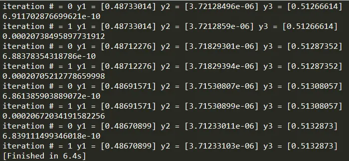
Here we can see that the iterations for y1, y2 & y3 and also the error for each iterations. Upto this iterations solution are converged. Error = 6.839e-10.

OBSERVATIONS :-

As the solution marches forward in time, the values change rapidly to different values. This behavior shows the stiff charecterastics of the given system.

As for the value of time step, 0.5 is used for solving this problem ut changing the time step does not seem to affect the results. Though if we give give a small value of time step the solution marches more forward in time as the end time remains the same and for a large value of time step the solution still remains stable and is able to converge and provide meaningful results.

The unconditional stability of the solution is due to the fact that we are using an Implicit scheme here which is stable irrespective of the time step value. Whereas the explicit schemes stability depends on the value of time-step.

Though explicit schemes are easy to solve compared to the implicit schemes.

CONCLUSIONS :-

As we have seen the above results at each time step getting an approximation value of (y1, y2, y3) and stable solution. If we change the time step but the solution has stable because using the implicit method (iterative method). But if you use an explicit method it’s depends on the step size and relaxation factor, step size is large error also large and relaxation factor greater than one it’s going to solution unstable.

More iteration needs tobe run for better accuracy in the results for simulation. Having the value of dt<0.1 provides accurate results for our simulation but there is a necessity for bringing down the time required for computations.

In this way I write the code and plot the figure and describe that why time step is so important.