ODE Using Multivariate Newton Raphson Method

AIM – To solve a system of coupled Ordinary Differential Equations using Multivariate Newton Raphson Method

THEORY –

Newton Raphson method for a single variable is used for root finding of non linear equations which are given as –

`f(x)=0`

It is an iterative method which approximates the value of x by linearizing f(x) i.e. approximating f(x) as a straight line. It’s general form for a nonlinear equation with a single variable is given as–

`x_(k+1)=x_k-(f(x_k))/(f'(x_k))`

Here `x_(k+1)` is the value of x at the next iteration while `x_k` is the value of x at current iteration (known).

This similar approach is extended to solve system of nonlinear equations. The method is then called as Multivariate Newton Raphson Method. In this method we solve iteratively a sequence of linear system of equations (linearized using the Newton’s Method).

Consider the following nonlinear coupled equations –

`f_1 (x_1,x_2,x_3,…..x_n )=0`

`f_2 (x_1,x_2,x_3,…..x_n )=0`

`f_n (x_1,x_2,x_3,…..x_n )=0`

The above equations can be written in matrix form as

`F(x)=[[f_1 (x)],[f_2 (x)],[f_3 (x)],[.],[.],[f_n (x)]]=[[0],[0],[0],[.],[.],[0]]=[0]`

In the above equation `x = x_1,x_2,x_3,…..x_n`. It must be noted that the number of variables and the number of nonlinear equations must be the same.

Extending the Newton Raphson Method for a single variable to the above multivariate equation set, we arrive at the form

`[[x_(1,k+1)],[x_(2,k+1)],[x_(3,k+1)],[.],[.],[x_(n,k+1)]] = [[x_(1,k)],[x_(2,k)],[x_(3,k)],[.],[.],[x_(n,k)]] - [[(∂f_1)/(∂x_1),(∂f_1)/(∂x_2 ),.,.,(∂f_1)/(∂x_n)],[(∂f_2)/(∂x_1),(∂f_2)/(∂x_2 ),.,.,(∂f_n)/(∂x_n)],[(∂f_3)/(∂x_1),(∂f_3)/(∂x_2 ),.,.,(∂f_3)/(∂x_n)],[.,.,.,.,.],[.,.,.,.,.],[(∂f_n)/(∂x_1),(∂f_n)/(∂x_2 ),.,.,(∂f_n)/(∂x_n)]]^-1.[[f_1(x_1,x_2,....x_n)],[f_2(x_1,x_2,....x_n)],[f_3(x_1,x_2,....x_n)],[.],[.],[f_n(x_1,x_2,....x_n)]]`

The above equation in matrices form can also be written as

`X_(k+1)=X_k-J^(-1) F(X_k)`

Where

`X_(k+1) = [[x_(1,k+1)],[x_(2,k+1)],[x_(3,k+1)],[.],[.],[x_(n,k+1)]]`

`X_k = [[x_(1,k)],[x_(2,k)],[x_(3,k)],[.],[.],[x_(n,k)]]`

Jacobian `J = [[(∂f_1)/(∂x_1),(∂f_1)/(∂x_2 ),.,.,(∂f_1)/(∂x_n)],[(∂f_2)/(∂x_1),(∂f_2)/(∂x_2 ),.,.,(∂f_n)/(∂x_n)],[(∂f_3)/(∂x_1),(∂f_3)/(∂x_2 ),.,.,(∂f_3)/(∂x_n)],[.,.,.,.,.],[.,.,.,.,.],[(∂f_n)/(∂x_1),(∂f_n)/(∂x_2 ),.,.,(∂f_n)/(∂x_n)]]`

`F(X_n ) = [[f_1(x_1,x_2,....x_n)],[f_2(x_1,x_2,....x_n)],[f_3(x_1,x_2,....x_n)],[.],[.],[f_n(x_1,x_2,....x_n)]]`

The above equation can be modified using an under relaxation factor. Thus the modified equation becomes -

`X_(k+1)=X_k-alphaJ^(-1) F(X_k)`

SOLVING A COUPLED SYSTEM OF ODE USING MULTIVARIATE NEWTON RAPHSON METHOD -

Many engineering processes (like chemical reacting systems) can be expressed as a system of ODEs. No computer can solve ordinary differential equations directly. Thus, first we need to convert the ordinary differential equations to algebraic equations using a suitable numerical method. This algebraic equation then becomes a nonlinear equation. Thus, the problem changes from solving ODEs to solving coupled nonlinear equations.

To convert an ordinary differential equation to an algebraic equation Backward Difference method (Implicit Euler Method) is employed. Then the multivariate newton Raphson method is employed to solve for the unknown variables iteratively.

The solution procedure can be understood with the following example.

`(dy_1)/dt= -0.04y_1+10^4 y_2 y_3`

`(dy_2)/dt= 0.04y_1-10^4 y_2 y_3-3*10^7 y_2^2`

`(dy_3)/dt= 3*10^7 y_2^2`

The above system of coupled ODEs can be converted to algebraic equations using the Backward Difference method. This is done to prevent stability issues, in case the system is stiff.

`(y_1^n-y_1^(n-1))/(Δt)= -0.04y_1+10^4 y_2 y_3`

`⇒y_1^n-y_1^(n-1)-dt*(-0.04y_1+10^4 y_2 y_3 )=f_1^n (y_1,y_2,y_3)`

Similarly

`⇒y_2^n-y_2^(n-1)-dt*(0.04y_1-10^4 y_2 y_3-3*10^7 y_2^2 )=f_2^n (y_1,y_2,y_3)`

`⇒y_3^n-y_3^(n-1)-dt*(3*10^7 y_2^2 )=f_3^n (y_1,y_2,y_3)`

Then using the Newton Raphson method, at each time step we need to solve the following equations for become

`⇒y_(1,k+1)^n=y_(1,k)^n-J_(f1) f_1 y_(1,k)^n`

`⇒y_(2,k+1)^n=y_(2,k)^n-J_(f2) f_2 y_(2,k)^n`

`⇒y_(2,k+1)^n=y_(2,k)^n-J_(f3) f_3 y_(3,k)^n`

In matrix form, the above sets of equations can be written as

`Y_(k+1)^n= Y_k^n-αJ^(-1) F(Y_k^n)`

Here, `Y_(k+1)^n` is the value of variables at the next iteration for the current time step (unknown).

`Y_k^n` is the value of variables at the current iteration for the current time step (known).

`alpha` is the under relaxation factor.

is the Jacobian matrix. It is calculated during each iteration using the values of the old iteration at that particular time step..

`F(Y_k^n)` is the value of nonlinear equation. It is calculated during each iteration using the values of the variables from the previous iteration.

While calculating J and F, it must be noted that the value of `y_1^(n-1),y_2^(n-1) and y_3^(n-1)` at each iteration level is constant for that time step. This value is the guess value at the start of each time step and must be updated after the iteration loop.

The solution algorithm is –

1. Defining the initial condition of each variable, total time and time step size.
2. For each time step, calculate the values of the Jacobian (using numerical differentiation) and the value of the functions (nonlinear equations) using the previous time step value and the old iteration values of the current time step
3. Using the Newton Raphson algorithm, calculate the new value of each variable from the old values of that time step and the previous time step values.
4. Update the old values with the new values at the end of each iteration.
5. Iterate till a desired tolerance criterion is met
6. At the end of each time step, update the previous time step values with that obtained from the current time step.
7. Repeat the steps 2 to 6 for the required time.

Results and discussions –

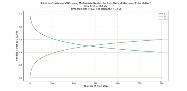
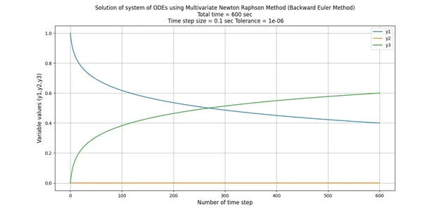
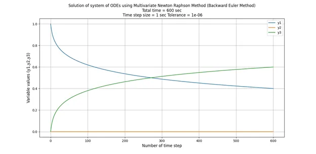
The system of ODEs was solved for y1, y2 and y3 at time step sizes of 0.01, 0.1 and 1 sec. The total time of simulation was 600 seconds. From the graphs above, it is clear that the time step size has negligible effect on the solution. However, it has major impact on the computational time. Computational time decreased significantly when time step size was increased from 0.01 sec to 1 sec. This is the major advantage of Implicit Euler’s method.

The values of y1, y2 and y3 highlight the most important characteristic of this system i.e. it is a stiff system of ODEs. The system is called stiff because the rate of change of one of the variables (y3) in this case is very less as compared to the other two variables. Such kind of systems are frequently observed in chemically reacting systems. Thus, if we obtain the rate equations of species in a chemical system, its variation with time can also be approximated using the same algorithm as discussed here.

After performing the computation at different time step sizes of .01 to 1 sec, it was concluded that 1 sec can be considered as the ideal time because of the least computational time required for the simulation. It must be noted that 1 sec can’t be considered as an ideal time step size of any system.

PYTHON CODE FOR SOLVING THE ODE SYSTEM

"""
Program to solve a system of non linear DE using the implicit Backward Euler method and multivariate NR method

dy1/dt = -0.04y1+10e4y2y3
dy2/dt = 0.04y1 -10e4y2y3 -3e7y2*y2
dy3/dt = 3e7y2*y2

Newton Raphson's multivariate method-
Y_new = Y_old -alpha*inv(J)*F(Y_old)

Implicit Euler's Method has been used (Backward)
i.e.
y1' = y1_n-y1_o = dt*RHS
=> f1 = y1_n-y1_o - dt*RHS
Similarly f2 and f3
"""

import numpy as np 
from numpy.linalg import inv
import matplotlib.pyplot as plt 

#Initial guess values of y1,y2 and y3 at time = 0. This is constant for each time step
y1_o = 1
y2_o = 0
y3_o = 0 

#Column vector to store the values for vectorization of the code. This changes during each iteration at that time step
Y_old = np.ones((3,1))
Y_old[0] = y1_o
Y_old[1] = y2_o
Y_old[2] = y3_o

#If we use = operator i.e. F = Y_old, when F changes in the loop, Y_old will also change, which we do not want.
#By using the copy function, Y_old doesn't change when F is updated in the loop

F = np.copy(Y_old)
Y_new = Y_old 

#Control values
tol = 1e-6
alpha = 1
t_start = 0
t_end = 10*60	#10 minutes 
dt = 1
n = int(t_end/dt)
t_steps = np.linspace(t_start,t_end,n+1)
#Storing the values at the end of each time step
y1_t = y1_o*np.ones((n+1,1))
y2_t = y2_o*np.ones((n+1,1))
y3_t = y3_o*np.ones((n+1,1))

def f1(y1_o,y1_n,y2_n,y3_n,dt):	#Defining the first non linear equation
	return y1_n-y1_o-dt*(-0.04*y1_n+10000*y2_n*y3_n)

def f2(y2_o,y1_n,y2_n,y3_n,dt):	#Defining the second non linear equation
	return y2_n-y2_o-dt*(0.04*y1_n-10000*y2_n*y3_n-3e07*pow(y2_n,2))

def f3(y3_o,y1_n,y2_n,y3_n,dt):	#Defining the third non linear equation
	return y3_n-y3_o-dt*(3e07*pow(y2_n,2))

def jacobian(y1_o,y2_o,y3_o,y1_n,y2_n,y3_n,dt):
	"""Returns the Jacobidan matrix using Forward differencing method
	Since the number of functions and variables are 3, thus the Jacobian matrix will be a 3x3 matrix
	"""
	h = 1e-06
	J = np.ones((3,3))
	#Row 1
	J[0,0] = (f1(y1_o,y1_n+h,y2_n,y3_n,dt)-f1(y1_o,y1_n,y2_n,y3_n,dt))/h
	J[0,1] = (f1(y1_o,y1_n,y2_n+h,y3_n,dt)-f1(y1_o,y1_n,y2_n,y3_n,dt))/h
	J[0,2] = (f1(y1_o,y1_n,y2_n,y3_n+h,dt)-f1(y1_o,y1_n,y2_n,y3_n,dt))/h

	#Row 2
	J[1,0] = (f2(y2_o,y1_n+h,y2_n,y3_n,dt)-f2(y2_o,y1_n,y2_n,y3_n,dt))/h
	J[1,1] = (f2(y2_o,y1_n,y2_n+h,y3_n,dt)-f2(y2_o,y1_n,y2_n,y3_n,dt))/h
	J[1,2] = (f2(y2_o,y1_n,y2_n,y3_n+h,dt)-f2(y2_o,y1_n,y2_n,y3_n,dt))/h

	#Row 3
	J[2,0] = (f3(y3_o,y1_n+h,y2_n,y3_n,dt)-f3(y3_o,y1_n,y2_n,y3_n,dt))/h
	J[2,1] = (f3(y3_o,y1_n,y2_n+h,y3_n,dt)-f3(y3_o,y1_n,y2_n,y3_n,dt))/h
	J[2,2] = (f3(y3_o,y1_n,y2_n,y3_n+h,dt)-f3(y3_o,y1_n,y2_n,y3_n,dt))/h

	return J

for t in range(1,n+1):
	itr = 1
	error = 1

	while (error>tol):
		#Calculating the Jacobian
		J = jacobian(y1_o,y2_o,y3_o,Y_old[0],Y_old[1],Y_old[2],dt)

		#Returning the values of the function at X_old
		F[0] = f1(y1_o,Y_old[0],Y_old[1],Y_old[2],dt)
		F[1] = f2(y2_o,Y_old[0],Y_old[1],Y_old[2],dt)
		F[2] = f3(y3_o,Y_old[0],Y_old[1],Y_old[2],dt)

		#Iteration update
		Y_new = Y_old - alpha*np.matmul(inv(J),F)

		error = max(abs(Y_new-Y_old))
		Y_old = Y_new
		print('time = {0}	iteration # = {1}	y1 = {2}	y2 = {3}	y3 = {4}'.format(t*dt,itr,Y_new[0],Y_new[1],Y_new[2]))
		itr = itr+1

	
	y1_t[t] = Y_new[0]
	y2_t[t] = Y_new[1]
	y3_t[t] = Y_new[2]
	#Updating the initial guess values for the next time step
	y1_o = Y_new[0]
	y2_o = Y_new[1]
	y3_o = Y_new[2]

#Plotting the results
plt.plot(t_steps,y1_t)
plt.plot(t_steps,y2_t)
plt.plot(t_steps,y3_t)
plt.xlabel('Number of time steps',fontsize=12)
plt.ylabel('Variable values (y1,y2,y3)',fontsize=12)
plt.legend(['y1','y2','y3'])
plt.title('Solution of system of ODEs using Multivariate Newton Raphson Method (Backward Euler Method)n Total time = {0} sec n Time step size = {1} sec Tolerance = {2}'.format(t_end,dt,tol))
plt.grid('on')
plt.show()