Multivariate Newton Raphson Solver
AIM
The aim of this project is to solve the system of ODE using Newton Raphson Method
MULTIVARIATE NEWTON RAPHSON SOLVER
Now lets discretise the equations which are being shown
`(y_1^(t) - y_1^(t-Delta t))/(Delta t) = -0.004 y_1^t + 10^4 y_2^t y_3^`
Rearranging the terms,
`y_1^(t) = y_1^(t-Delta t) + Delta t(-0.004 y_1^t + 10^4 y_2^t y_3^t)`
`y_2^t = y_2^(t-Delta t) + Delta t(0.004 y_1^t - 10^4 y_2^t y_3^t - 3*10^7 (y_2^t)^2)`
`y_3^t = y_3^(t-Delta t) + Delta t (3*10^7 (y_2^t)^2)`
For solving this equations using the multivariate newton Raphson method, it must be converted to root finding problem. Hence we obtain
`y_1^(t-Delta t) + Delta t(-0.004 y_1^t + 10^4 y_2^t y_3^t) - y_1^(t) = 0`
`y_2^(t-Delta t) + Delta t(0.004 y_1^t - 10^4 y_2^t y_3^t - 3*10^7 (y_2^t)^2) - y_2^t = 0`
`y_3^(t-Delta t) + Delta t (3*10^7 (y_2^t)^2) - y_3^t = 0`
NEWTON RAPHSON SOLVER
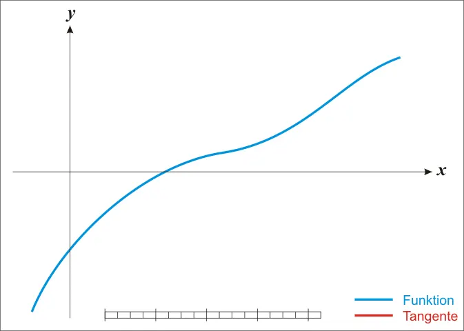
The idea is to start with an initial guess which is reasonably close to the true root, then to approximate the function by its tangent line using calculus, and finally to compute the x-intercept of this tangent line by elementary algebra. This x-intercept will typically be a better approximation to the original function's root than the first guess, and the method can be iterated.
More formally, suppose f : (a, b) → ℝ is a differentiable function defined on the interval (a, b) with values in the real numbers ℝ, and we have some current approximation xn. Then we can derive the formula for a better approximation, xn + 1 by referring to the diagram on the right. The equation of the tangent line to the curve y = f (x) at x = xn is

where f′ denotes the derivative. The x-intercept of this line (the value of x which makes y = 0) is taken as the next approximation, xn + 1, to the root, so that the equation of the tangent line is satisfied when

Solving for xn + 1 gives

We start the process with some arbitrary initial value x0. (The closer to the zero, the better. But, in the absence of any intuition about where the zero might lie, a "guess and check" method might narrow the possibilities to a reasonably small interval by appealing to the intermediate value theorem.) The method will usually converge, provided this initial guess is close enough to the unknown zero, and that f ′(x0) ≠ 0. Furthermore, for a zero of multiplicity 1, the convergence is at least quadratic (see rate of convergence) in a neighbourhood of the zero, which intuitively means that the number of correct digits roughly doubles in every step. More details can be found in the analysis section below.
Householder's methods are similar but have higher order for even faster convergence. However, the extra computations required for each step can slow down the overall performance relative to Newton's method, particularly if f or its derivatives are computationally expensive to evaluate.
In order to apply the Newton Raphson method
`y^(n+1) = y^n - alpha f(x)/(f'(x))`
`y^n`is the old value
`y^(n+1)`is the new value
`alpha`is the relaxation factor
`f(x)`is the original function
`f'(x)`is the first derivative of the function
Since there are 3 equations with three unknowns we have to use the multivariate newton raphson method
`[Y]^(n+1)= [Y]^n-alphaJ^(-1)F`
So lets see how we can evaluate the terms from the above equation
`[Y]^n={[y_1^(n)],[y_2^(n)],[y_3^(n)]}`
`[Y]^(n+1)={[y_1^(n+1)],[y_2^(n+1)],[y_3^(n+1)]}`
`J = {[frac[delf_1][dely_1},frac[delf_1][dely_2],frac[delf_1][dely_3]],[frac[delf_2][dely_1],frac[delf_2][dely_2],frac[delf_2][dely_3]],[frac[delf_3][dely_1],frac[delf_3][dely_2],frac[delf_3][dely_3]]}`
MULTIVARIATE NEWTON RHAPSON CODE
import matplotlib.pyplot as plt
from numpy.linalg import inv
import numpy as np
def f1(y10,y1,y2,y3,dt):

	return (y10 + dt*(-0.04*y1 + y2*y3*1e4) - y1)

def f2(y20,y1,y2,y3,dt):

	return (y20 + dt*(0.04*y1 - (1e4*y2*y3) -(3e7*y2*y2)) -y2)

def f3(y30,y1,y2,y3,dt):

	return (y30 + dt*(3e7*y2*y2) - y3)

def jacobian(y10,y20,y30,y1,y2,y3,dt):
	J = np.ones((3,3))
# Jacobian solved by numerical derivative.
	h = 1e-6 # Step size

	J[0,0] = (f1(y10,y1+h,y2,y3,dt)-f1(y10,y1,y2,y3,dt))/h
	J[0,1] = (f1(y10,y1,y2+h,y3,dt) -f1(y10,y1,y2,y3,dt))/h
	J[0,2] = (f1(y10,y1,y2,y3+h,dt) -f1(y10,y1,y2,y3,dt))/h

	#Row 2
	J[1,0] = (f2(y20,y1+h,y2,y3,dt) -f2(y20,y1,y2,y3,dt))/h
	J[1,1] = (f2(y20,y1,y2+h,y3,dt) -f2(y20,y1,y2,y3,dt))/h
	J[1,2] = (f2(y20,y1,y2,y3+h,dt)-f2(y20,y1,y2,y3,dt))/h
# Row 3
	J[2,0] = (f3(y30,y1+h,y2,y3,dt)-f3(y30,y1,y2,y3,dt))/h
	J[2,1] = (f3(y30,y1,y2+h,y3,dt)-f3(y30,y1,y2,y3,dt))/h
	J[2,2] = (f3(y30,y1,y2,y3+h,dt)-f3(y30,y1,y2,y3,dt))/h
	return J
# Defining initial guess value
y10 = 1
y20 = 0
y30 = 0
# Initial error
error = 9e9
#Column Vector
Y_old = np.ones((3,1))
Y_old[0] = y10
Y_old[1] = y20
Y_old[2] = y30
# Column Vectors for F
F = np.copy(Y_old)
#Parameters for newton rapson method
alpha = 1
tol = 1e-6
t = 600
dt = 0.1
n = int(t/dt)
x1 = []
x2 = []
x3 = []
iteration = []

iter = 1
for i in range(0,n):
	while error>tol:
		J = jacobian(y10,y20,y30,Y_old[0],Y_old[1],Y_old[2],dt)
# Computing the F vector
		F[0] = f1(y10,Y_old[0],Y_old[1],Y_old[2],dt)
		F[1] = f2(y20,Y_old[0],Y_old[1],Y_old[2],dt)
		F[2] = f3(y30,Y_old[0],Y_old[1],Y_old[2],dt)
# Computing the new values
		Y_new = Y_old - alpha*np.matmul(inv(J), F)
		error = max(abs(Y_new-Y_old))
		print(error) #Updating the old values
		Y_old = Y_new #log message
# Storing the values for plotting
		x1.append(Y_new[0])
		x2.append(Y_new[1])
		x3.append(Y_new[2])
		iter = iter + 1
		iteration.append(iter)
		Y_old = Y_new
		y10 = Y_new[0]
		y20 = Y_new[1]
		y30 = Y_new[2]

plt.plot(iteration,x1, color = 'green')
plt.plot(iteration,x2, color = 'red')
plt.plot(iteration,x3, color = 'black')
plt.xlabel('Number of Iterations')
plt.ylabel('Variables')
plt.legend(['y1','y2','y3'])
plt.title('Solution for ODE System')
plt.grid()
plt.show()
In the beginning of the program, the required libraries and imorted and the 3 functions f1,f2 and f3 are defined. Then we introduce the jacobian matrix function and define the formulas for the respective rows and columns. Then we say the initial conditions
y10 = 1
y20 = 0
y30 = 0
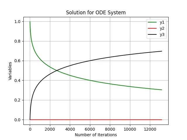
Now we define these values in the current time step as Y_old. Next we create the function vector f1,f2 and f3. The next time step is defined by saying Y_new values for the solution of variables in the ODE system. Then we create empty arrays x1,x2 and x3 to store the values of the solutions computed by the program.We define the tolerance and error parameters, then the while condition is employed till the error is greater than the tolerance the solution will take place. The update rule is created by the statement Y_new = Y_old. The results are plotted as shown below
As we can observe the time step taken in the program is 0.1 to get stable solution. We are using the implicit scheme of integration to solve the equations. The time step does not affect the solution because the implicit scheme is quiet stable over a large values of time steps.
PLOT FOR THE CODE
CONCLUSION
- The system of equations were solved using the multivariate newton rhapson method
- The implicit solution has no effect on the time step
- The plot shows the trend for how the equations behave in cartesian plane