Week 6 - Multivariate Newton Rhapson Solver

Aim :

we will solving the given coupled non-linera equations using multivariatae newton raphson method

Theory:

from the given set of differential equations,these equations are interdependent variables and these equations can be solved by using multivariatae newton raphson method

#dy1/dt = -0.04*y1+10^4*y2*y3
#dy2/dt = 0.04*y1-10^4*y2*y3-3*10^7*y2*y2
#dy3/dt = 3*10^7*y2*y2

import numpy as np
from numpy.linalg import inv
import matplotlib.pyplot as plt

def f1(y1_old,y1,y2,y3,dt):
# first non-linear equation
return (y1_old+dt*(-0.04*y1+y2*y3*pow(10,4))-y1)

def f2(y2_old,y1,y2,y3,dt):
#secon non-limear equation
return (y2_old+dt*(0.04*y1-(pow(10,4)*y2*y3)-(3*pow(10,7)*pow(y2,2)))-y2)

def f3(y3_old,y1,y2,y3,dt):
#third non-linear equation
return (y3_old+dt*(3*pow(10,7)*pow(y2,2))-y3)

def jacobian(y1_old,y2_old,y3_old,y1,y2,y3,dt):
# defining the jacobian

J = np.ones((3,3))

#row1
h = 1e-5

J[0,0] = (f1(y1_old,y1+h,y2,y3,dt)-f1(y1_old,y1,y2,y3,dt))/h
J[0,1] = (f1(y1_old,y1,y2+h,y3,dt)-f1(y1_old,y1,y2,y3,dt))/h
J[0,2] = (f1(y1_old,y1,y2,y3+h,dt)-f1(y1_old,y1,y2,y3,dt))/h

#row2

J[1,0] = (f2(y2_old,y1+h,y2,y3,dt)-f2(y2_old,y1,y2,y3,dt))/h
J[1,1] = (f2(y2_old,y1,y2+h,y3,dt)-f2(y2_old,y1,y2,y3,dt))/h
J[1,2] = (f2(y2_old,y1,y2,y3+h,dt)-f2(y2_old,y1,y2,y3,dt))/h

#row3

J[2,0] = (f3(y3_old,y1+h,y2,y3,dt)-f3(y3_old,y1,y2,y3,dt))/h
J[2,1] = (f3(y3_old,y1,y2+h,y3,dt)-f3(y3_old,y1,y2,y3,dt))/h
J[2,2] = (f3(y3_old,y1,y2,y3+h,dt)-f3(y3_old,y1,y2,y3,dt))/h

return J

# defining the initial guess values

y1_old = 1
y2_old = 0
y3_old = 0

#initial erroe
error = 9e9

y_old = np.ones((3,1))
y_old[0] = y1_old
y_old[1] = y2_old
y_old[2] = y3_old

#numpy
f = np.copy(y_old)

tol = 0.01
alpha = 1
t = 600
dt = 1
n = int(t/dt)

y_1 = []
y_2 = []
y_3 = []
iteration = []
iter = 1

for i in range(0,n):
while error>tol:
J = jacobian(y1_old,y2_old,y3_old,y_old[0],y_old[1],y_old[2],dt)

f[0] = f1(y1_old,y_old[0],y_old[1],y_old[2],dt)
f[1] = f2(y2_old,y_old[0],y_old[1],y_old[2],dt)
f[2] = f3(y3_old,y_old[0],y_old[1],y_old[2],dt)

y_new = y_old - alpha*np.matmul(inv(J),f)
error = np.max(np.abs(y_new-y_old))

# updating old values
y_old = y_new;

log_message = 'iteration number = {0} y1={1} y2 = {2} y3 = {3}' .format(iter,y_new[0],y_new[1],y_new[2])
print(log_message)

iter = iter+1

y_old = y_new
y1_old = y_new[0]
y2_old = y_new[1]
y3_old = y_new[2]

y_1.append(y_new[0])
y_2.append(y_new[1])
y_3.append(y_new[2])

iteration.append(iter)
error = 9e9
plt.plot(iteration,y_1,color = 'green')
plt.plot(iteration,y_2,color = 'red')
plt.plot(iteration,y_3,color = 'black')
plt.xlabel('no of steps')
plt.ylabel('variable species')
plt.legend(['y_1','y_2','y_3'])
plt.title('multivariate newton rphson method')
plt.show()

output:

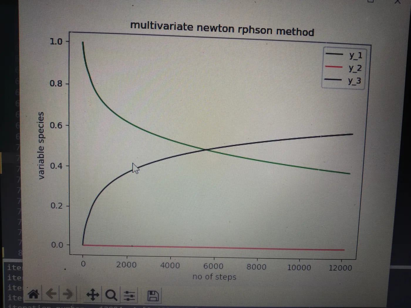
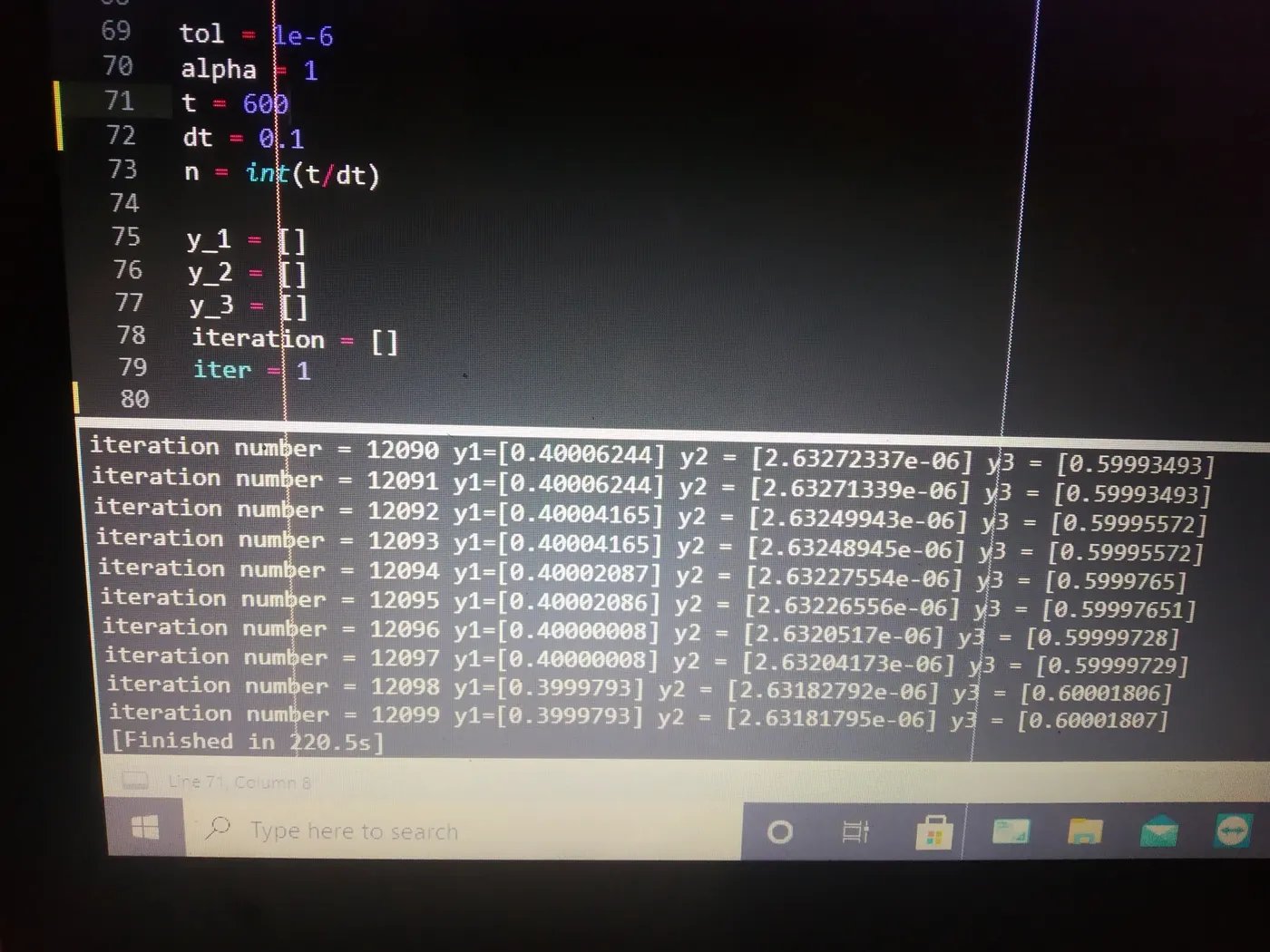
n = 6000 and dt = 0.1

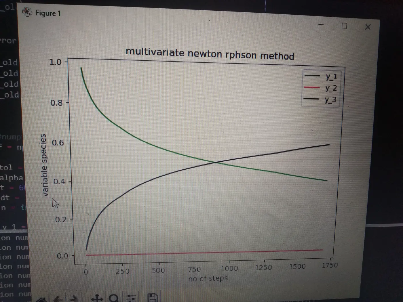
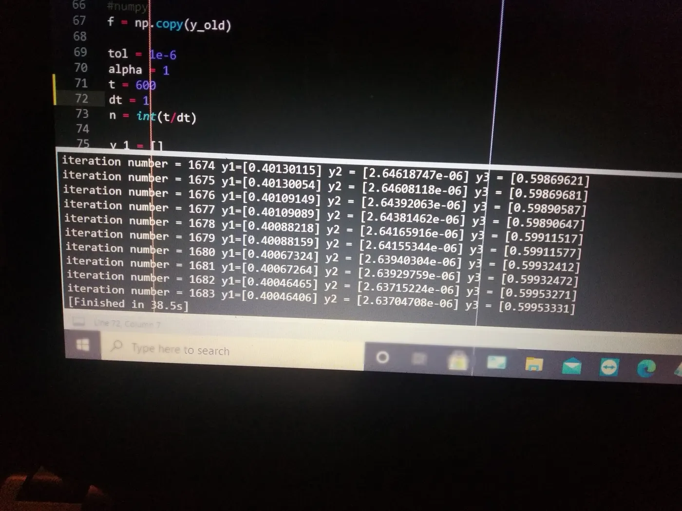
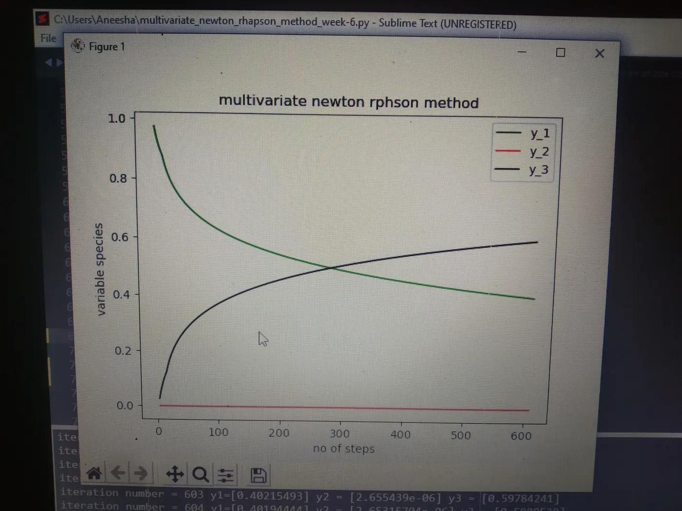
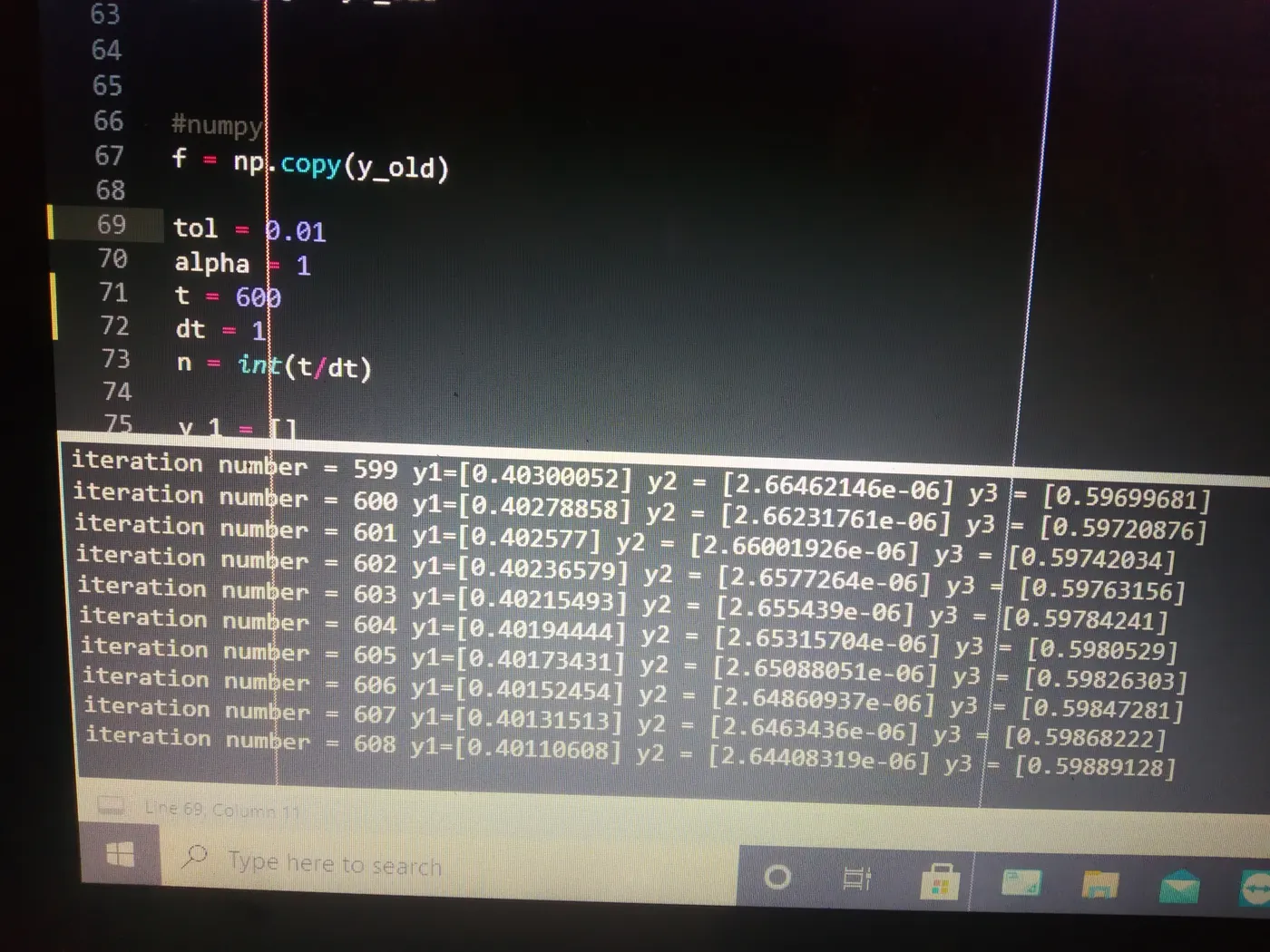
n = 600 and dt = 1

n = 60000 and dt = 0.01

result:

from the graphs we can say that valus of y1,y2,y3 are changeing with respective time.for the vlues of y2 we cannot find any change as y2 value is small.

the value of timestep used in above cases are 0.1,1,0.01. as we decreases the time step value , n increases ,as for results concerned there is not much of difference in the obtained value .