Multivariate Newton Rhapson Solver

Objectives:

1. Solve the given set of coupled Ordinary Differential Equations (ODEs), implicitly, using multivariate Newton Rhapson technique
2. Find the effect of time step on stability of the system

The given ODEs are,

`(dy_1)/(dt) = -0.04y_1 + 10^4y_2_y3`

`(dy_2)/(dt) = 0.04y_1 - 10^4y_2y_3 - 3*10^7y_2^2`

`(dy_3)/(dt) = 3*10^7y_2^2`

Theory:

Mathematical methods, which are used to solve equations or evaluate integrals or solve differential equations can be classified broadly into two types,

1. Analytical methods
2. Numerical methods

Analytical methods are those which by an analysis of the equation obtain a solution directly by the application of formulae. In numerical solution, instead of directly writing the answer, stepwise calculations using some algorithms or numerical procedures are performed and arrive at the same results.

The advantage of numerical methods is that usually these procedures work on a much wider range of problems as compared to analytical solutions which work only on a limited class of problems.

Differential equations are solved numerically by several methods, some of them are,

1. Euler's method (explicit scheme)
2. Modified Euler's method (implicit scheme)
3. Range - Kutta method

In this case, modified Euler's method is used.

Euler's method:

Consider a differential equation of form, `(dy)/(dx) = f(x,y)`

The above `f(x,y)` curve is plotted and the x-axis is divided into many number of sub intervals with interval length dx. Then the points would be, `x_0, x_0 + dx, x_0 + 2dx...`

In Euler's method the curve is considered linear along the length of this sub interval.

Now, by using elementary algebra, the projection of `x_0+dx` on the curve can be found and is given by the expression,

`y_1 = y_0 + dx*f(x_0,y_0)`

This can be generalised and can be written as,

`y_(n+1) = y_n + dx*f(x_n,y_n)`

The disadvantage with this method is that when the length of subinterval is small, the error is low and the system will be stable, that is when the number of sub intervals is large, when their number is small, dx would be large, error would be high and so the system becomes unstable.

To overcome this, Euler's method is modified, which is called as modified Euler's method, whose generaliazed expression is given by,

`y_(n+1) = y_n + dx*f(x_(n+1),y_(n+1))`

Notice that the modified Euler's method is implicit nature (`y_(n+1)` is on both LHS and RHS) and Euler's method is explicit. Implicit schemes are stable even at large values of length of sub intervals.

In Engineering, we often require to find the roots of the equations of the form f(x) = 0, which are called 'root finding problems'. There are several numerical methods to find the roots of such equations, which are,

1. Bisection method
2. Regula-Falsi method
3. Secant method
4. Newton-Raphson method

Each of these methods have their own advantages and disadvantages, however Newton Raphson method has the highest order of accuracy, 2.

Newton Raphson method:

Let us consider an equation f(x) = 0. Let `x_0` be an approximate root for the equation, and let `x_1 = x_0 + h` be the correct root (`h rightarrow 0`), then by expanding `f(x_0 + h)` using Taylor's series expansion,

`f(x_0+h) = f(x_0) + hf^I(x_0) + (h^2)/(2!) f^(II)(x_0)+...`

Now, as `x_0 + h` is the root, the LHS of the above expression would be zero. After neglecting the higher powers of h (degree 2), we get,

`h = -f(x_0)/f^I(x_0)` Now, the root then would become,

`x_1 = x_0 - f(x_0)/f^I(x_0)`

Generalising the above expression, which gives,

`x_(n+1) = x_n - f(x_n)/f^I(x_n)`

Geometrically, in Newton - Raphson method, a tangent to curve is drawn at point `(x_0,f(x_0))` and the point of intersection of this line and x-axis is `x_1`. Obviously, `x_1` is closer to root than `x_0`.

The method converges rapidly to the root with a second order convergence.

Introduction:

In this case, the give system of ODEs are solved using modified Euler's method (implicit scheme), which results in equations of form f(x) = 0, which are then solved using Newton Rhapson technique.

In this case, in the process of solving the give ODEs, equations which have more than two dependent variables are involved, which require 'multivariate Newton Rhapson method'. In multivariate Newton Rhapson method, the generalized expression is,

`Y_(n+1) = Y_n - alpha*J^(-1)*F`, where `alpha` is a relaxation factor (the value of which in this case is 1), F is function matrix, which stores the values of function at that particular time step and J is Jacobian matrix.

(A Jacobian matrix stores the change of each variable in all directions of considered coordinate system).

The matrix form of the above equation is,

`[[y_1^(n+1)],[y_2^(n+1)],[y_3^(n+1)]] = [[y_1^(n)],[y_2^n],[y_3^n]]-alpha*[[(deltaf_1)/(deltay_1),(deltaf_1)/(deltay_2),(deltaf_1)/(deltay_3)],[(deltaf_2)/(deltay_1),(deltaf_2)/(deltay_2),(deltaf_2)/(deltay_3)],[(deltaf_3)/(deltay_1),(deltaf_3)/(deltay_2),(deltaf_3)/(deltay_3)]]^(-1)*[[F_1^(n+1)],[F_2^(n+1)],[F_3^(n+1)]]`

Multivariate Newton Rhapson technique is similar to the normal one mentioned above, it also contains a differential term (rate of change of dependent variable with an independent variable), and the value of function at that time step.

As implicit scheme is used, the system will be stable even at large values of time step (length of sub interval). Ofcourse, there is a limitation to the length of time step, even for implicit scheme, which relatively is larger than the corresponding value for explicit scheme. That will be addressed in below sections.

The ODEs in this case are 'coupled ODEs' as each variable is linked with all of them and each has its own derivative term.

The variables involved in this case are `y_1, y_2 and y_3`. The initial values are 1, 0 and 0 for `y_1, y_2 and y_3` respectively.

Code:

Python code to solve the given set of coupled ODEs using multivariate Newton Rhapson technique is,

import matplotlib.pyplot as plt
import numpy as np
from numpy.linalg import inv


def f1(h,y1_old,y1,y2,y3):
	return y1_old + h*(-0.04*y1 + pow(10,4)*y2*y3) - y1

def f2(h,y2_old,y1,y2,y3):
	return y2_old + h*(0.04*y1 - pow(10,4)*y2*y3 - 3*pow(10,7)*pow(y2,2)) - y2

def f3(h,y3_old,y1,y2,y3):
	return y3_old + h*(3*pow(10,7)*pow(y2,2)) - y3

def Jac(h,y1_old,y2_old,y3_old,y1,y2,y3):
	dh = 1e-5

	J = np.ones((3,3))

	J[0,0] = (f1(h,y1_old,y1+dh,y2,y3) - f1(h,y1_old,y1,y2,y3))/(dh)
	J[0,1] = (f1(h,y1_old,y1,y2+dh,y3) - f1(h,y1_old,y1,y2,y3))/(dh)
	J[0,2] = (f1(h,y1_old,y1,y2,y3+dh) - f1(h,y1_old,y1,y2,y3))/(dh)

	J[1,0] = (f2(h,y2_old,y1+dh,y2,y3) - f2(h,y2_old,y1,y2,y3))/(dh)
	J[1,1] = (f2(h,y2_old,y1,y2+dh,y3) - f2(h,y2_old,y1,y2,y3))/(dh)
	J[1,2] = (f2(h,y2_old,y1,y2,y3+dh) - f2(h,y2_old,y1,y2,y3))/(dh)

	J[2,0] = (f3(h,y3_old,y1+dh,y2,y3) - f3(h,y3_old,y1,y2,y3))/(dh)
	J[2,1] = (f3(h,y3_old,y1,y2+dh,y3) - f3(h,y3_old,y1,y2,y3))/(dh)
	J[2,2] = (f3(h,y3_old,y1,y2,y3+dh) - f3(h,y3_old,y1,y2,y3))/(dh)

	return J

t_start = 0
t_end = 600 #Seconds
n = 1000
h = (t_end-t_start)/(n)

tol = 1e-5
alpha = 1

y1 = 1
y2 = 0
y3 = 0

var1 = []
var2 = []
var3 = []
time = np.linspace(t_start,t_end,n)

for i in range(0,n):

	y_old = np.ones((3,1))

	y_old[0] = y1
	y_old[1] = y2
	y_old[2] = y3

	y_guess = np.copy(y_old)
	F = np.copy(y_old)
	y_new = np.copy(y_old)

	error = 9e9
	ite = 1

	while error > tol:

		#JACOBI
		J = Jac(h,y_old[0],y_old[1],y_old[2],y_guess[0],y_guess[1],y_guess[2])

		F[0] = f1(h,y_old[0],y_guess[0],y_guess[1],y_guess[2])
		F[1] = f2(h,y_old[1],y_guess[0],y_guess[1],y_guess[2])
		F[2] = f3(h,y_old[2],y_guess[0],y_guess[1],y_guess[2])

		y_new = y_guess - alpha*np.matmul(inv(J),F)

		error = np.max(np.abs(y_guess - y_new))
		y_guess = y_new
		ite = ite + 1
		log_message = 'Iteration - {0}; y1 = {1}, y2 = {2}, y3 = {3}'.format(ite,y_new[0],y_new[1],y_new[2])
		print(log_message)

	var1.append(y_new[0])
	var2.append(y_new[1])
	var3.append(y_new[2])

	y1 = y_new[0] 
	y2 = y_new[1]
	y3 = y_new[2]

plt.plot(time,var1,color='blue')
plt.plot(time,var2,color='red')
plt.plot(time,var3,color='green')
plt.xlabel('Time (seconds)')
plt.ylabel('Variable value')
plt.title('Variation of values of y1, y2 and y3 with time')
plt.legend(['y1','y2','y3'])

print(time)
plt.show()

Results:

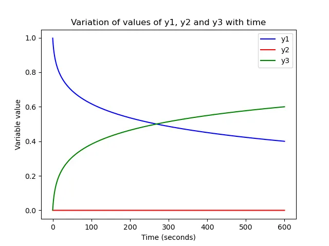
When the above code is executed, the resultant plot is,

NOTE: The step size (dt) value is 0.6 seconds (number of sub intervals, 1000)

Inferences:

• The values of both `y_1 and y_3` are changing more rigorously than `y_2`, which is varying almost constantly with time. This phenomenon of one term varying at a different rate than the other in the same system of equations is called as 'stiffness'. This stiffness arises because of the co-existence of a very fast reaction and very slow reaction
• In the current case, both terms `y_1` and `y_3` are changing rapidly in contrast to `y_2` which is almost constant. The safest explanation for this would be, in both ODEs for `y_1 and y_3`, when looked at, have positive terms multiplied with large values like `10^4 and 10^7`, so their time rate of change is faster than `y_2`
• In this case, we can have a relatively large time step for `y_2` and very small time step for `y_1 and y_3`

Even though implicit scheme is stable even at large values of time step or less number of sub intervals, it becomes unstable at very large values of time steps.

A. At time step value 1:

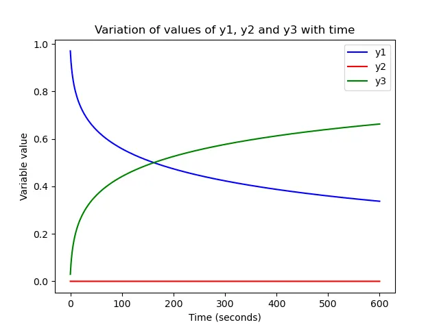
• Values of `y_1 and y_3` are starting to change early than when the time step value is small (like above)

B. At time step value 3:

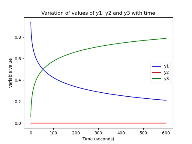
• The values are starting to change even more early than in the previous case

C. At time step value 5:

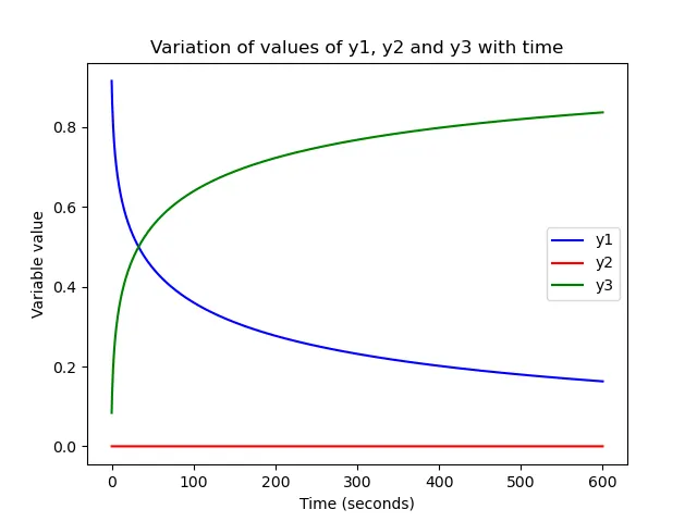
D. At time step values larger:

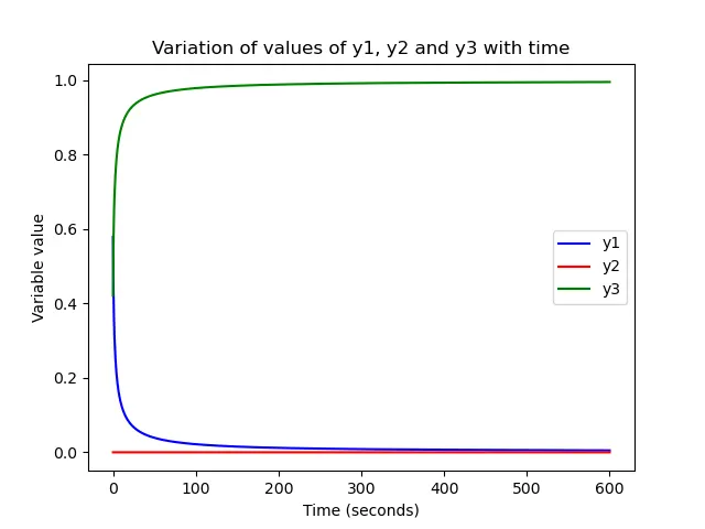
• When the time step value is higher (50 in this case), the values of `y_1 and y_3` are changing right at the beginning of simulation. Note that all these simulations are using implicit scheme only. And all the time rate of change of value of `y_2` remained constant in contrast to the others
• So even for implicit schemes, the time step value is to be checked for

Conclusions:

1. The given set of ODEs are solved using implicit Euler's method and multivariate Newton Rhapson technique
2. The effect of time step value is relatively small in case of implicit scheme, when compared with explicit scheme, but at large values of time step, even implicit scheme becomes unstable. However, for a given range of time step values, the changes are small when the value of time step is small (relatively). So depending on the problem and the level of stability needed, the time step value can be chosen, for this case

Appendix:

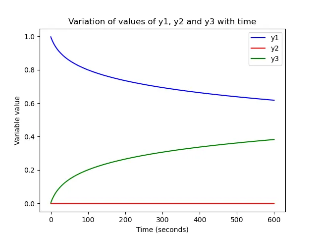
A. When the time step value is 0.1:

B. When the time step value is 0.01:

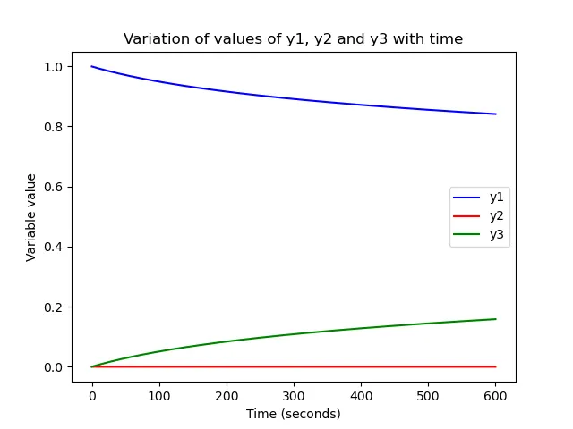
NOTE: Though the variation is not rapid when the time step is small, the load on the machine would be very high as number of time steps increases. For instance, for time step value 0.01, number of time steps needed are 60,000. So it is up to the level of stability we need and the problem, the required time step can be chosen.